

This article is written for beginners who have never written SQL before. We will learn all the essential SQL commands, from CREATE (create databases/tables), INSERT (add data), SELECT (retrieve data), UPDATE (modify data), all the way to DELETE (remove data), with hands-on examples you can follow along with.
First, let’s get to know four terms that we will use throughout the article:
- Database — like a “folder” or a “ledger” that holds tables inside it
- Table — like a “spreadsheet in Excel,” it has both rows and columns. For example, the
patienttable stores patient information - Row / record — the data of a single person or thing, one unit. For example, one patient’s data = 1 row
- Column — the same type of data throughout the column. For example, the
weightcolumn stores only weights
As for SQL (pronounced “S-Q-L” or “sequel”), it is the language we use to “talk” to the database — like giving instructions to an employee. For example, you might say “Show me the list of patients who weigh over 100 kilograms” — this sentence can be translated into SQL, and we will learn how to write it step by step.
In this article we will learn in order: install CAMPP → open phpMyAdmin → use CREATE to build a database and tables → use INSERT to add data → use SELECT to retrieve data (with WHERE, ORDER BY, GROUP BY, JOIN) → and use UPDATE to modify and DELETE to remove data.
Don’t worry if you don’t understand everything immediately — try typing the commands for real on your machine and look at the results. You will understand much faster than just reading.
1. Install CAMPP#
Before we can work with a database, we need a program that actually is a database. CAMPP is a free program that bundles the necessary tools into a single package. Think of it as a “toolbox” that is ready to use the moment you open it — no need to install each tool separately.
Inside CAMPP there are two important things we will use:
- MySQL / MariaDB — the actual database engine (the tool that stores the data)
- phpMyAdmin — a graphical (web) interface that lets us manage the database by clicking or typing SQL conveniently
Steps:
-
Download and install CAMPP from https://campp.melivecode.com/ ↗

-
Open the CAMPP program, then press the Start button to start the services.

After pressing Start, notice that each service shows a status of “running” (green) — meaning it is ready to use. If any service is not running, press Stop and then press Start again.
2. Open phpMyAdmin#
Although MySQL is the engine that stores the data, it does not provide a nice graphical interface to click. Talking to it directly through the command line is quite difficult for beginners. phpMyAdmin is like a “remote control” that lets us control the database easily through a web page.
You can open phpMyAdmin in two ways:
-
Click the phpMyAdmin button on the CAMPP web page
-
Open your browser and type this address: http://127.0.0.1:8080/phpmyadmin/ ↗
(
127.0.0.1is your own computer, and8080is the port — like the room number where this web page lives)
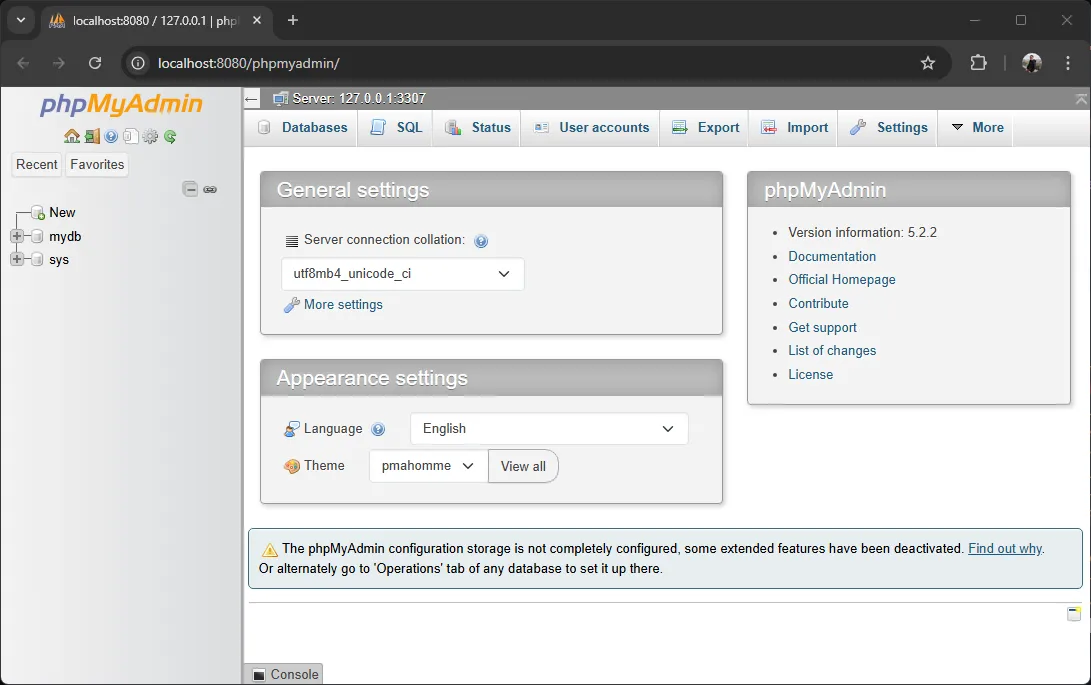
In phpMyAdmin you can manage the database in two ways:
- Option 1 — click through the GUI (graphical interface) — good for simple tasks like creating a database
- Option 2 — click the SQL tab and type the commands yourself — faster and more powerful. All the commands in this article we will run through this SQL tab
Why learn to type SQL yourself when there is a GUI to click? Because in real work, SQL commands can be saved inside programs, sent for applications to run, and can do far more complex things than clicking.
3. CREATE DATABASE — create a database#
Let’s start by creating the “folder” that will hold our tables. We’ll name it testdb.
-- Create a database (use IF NOT EXISTS so it doesn't error if it already exists)
CREATE DATABASE IF NOT EXISTS testdb;

-- Select the database to work with
USE testdb;Line-by-line explanation:
CREATE DATABASE— tells the database to “create a new database”IF NOT EXISTS— “only create it if it doesn’t already exist.” This prevents an error when we run the command repeatedly (e.g., on a second run, the database already exists — normally an error, but with this clause it is skipped)USE testdb;— “from now on, use the testdb database” — so the following commands land in the correct database
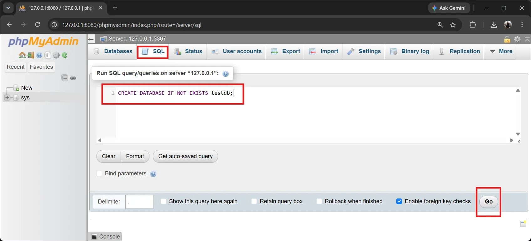
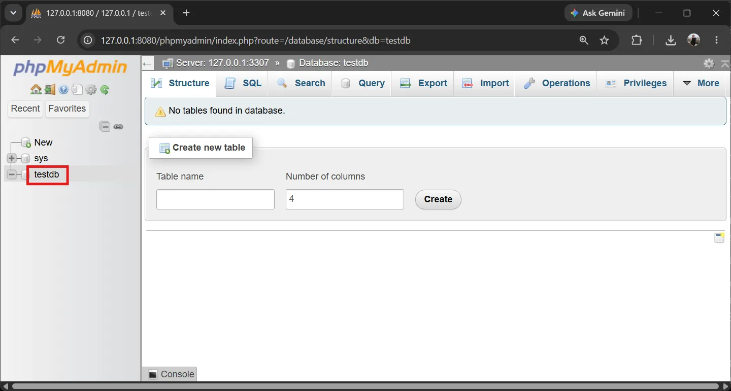
Note: A SQL command always ends with a semicolon
;— like a period at the end of a sentence that says “the statement is finished.” If you type only a single command and forget it, often it won’t error — but if you type several commands together, you must separate them with;
4. CREATE TABLE — create a table#
A table is like a spreadsheet in Excel: the first row is the “header” (column names), and the rows below are the data. What’s different from Excel is that when you create a table you must tell the database upfront what kind of data each column will hold — this is called the datatype.
Here are the commonly used datatypes:
| Datatype | What it stores | Examples |
|---|---|---|
INT | Whole numbers | ID, age, count |
VARCHAR(n) | Short text (up to n characters) | name, address, email |
DATE | A date in YYYY-MM-DD format | date of birth |
DECIMAL(p,s) | Decimal numbers that need precision | weight, price, money |
Why define a datatype? So the database can store the value correctly, save space, and search faster. If the
weightcolumn is defined asINT(a whole number), entering105.50will be truncated to just105— the decimal part is lost.
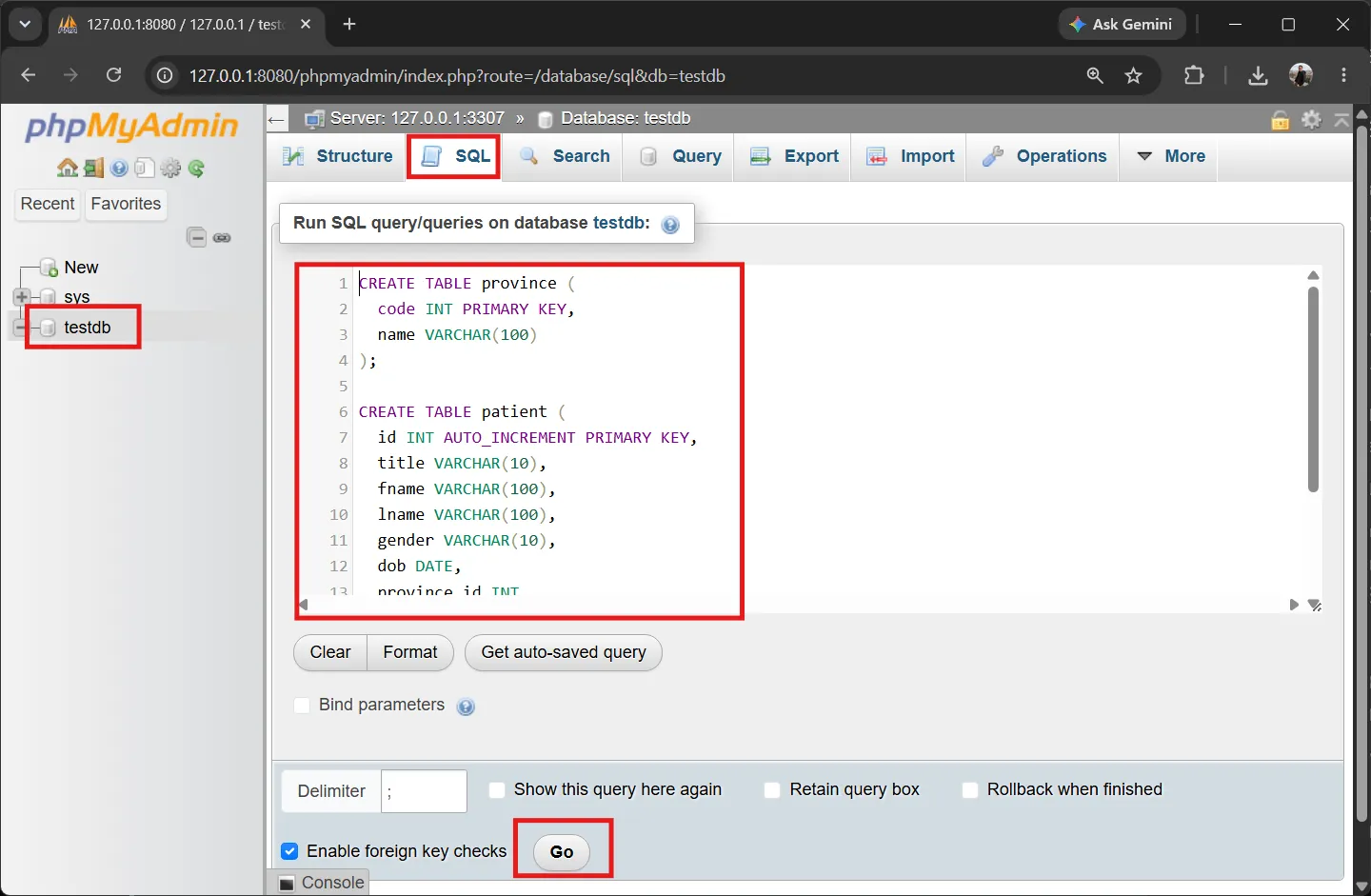
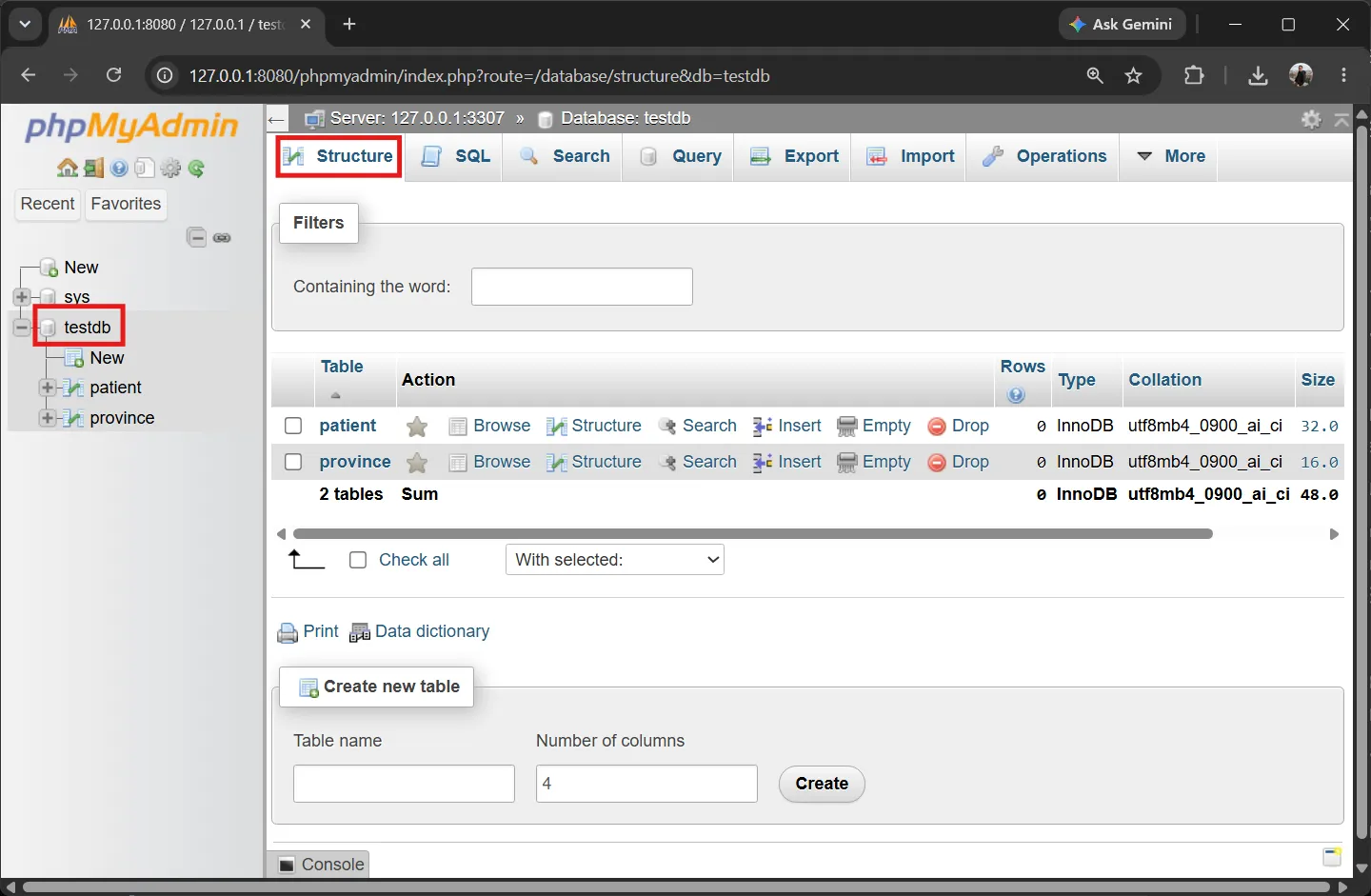
We will create 2 tables: province (stores provinces) and patient (stores patients).
-- province table (stores province data)
CREATE TABLE province (
  code INT PRIMARY KEY,
  name VARCHAR(100)
);

-- patient table (stores patient data)
CREATE TABLE patient (
  id INT AUTO_INCREMENT PRIMARY KEY,
  title VARCHAR(10),
  fname VARCHAR(100),
  lname VARCHAR(100),
  gender VARCHAR(10),
  dob DATE,
  province_id INT,
  weight DECIMAL(5,2),
  height DECIMAL(5,2),
  FOREIGN KEY (province_id) REFERENCES province(code)
);
There are three keywords you need to understand:
PRIMARY KEY— the “ID card” of each row. It makes each row unique and quick to look up- In
provinceit iscode(e.g., 10 = Bangkok) - In
patientit isid(1, 2, 3, …)
- In
AUTO_INCREMENT— tells the database to “count the number for us” (1, 2, 3, …) each time new data is added, so we don’t have to type the ID ourselvesFOREIGN KEY— like a “link” that connects one table to anotherFOREIGN KEY (province_id) REFERENCES province(code)means: theprovince_idcolumn in thepatienttable points tocodein theprovincetable- The result is that we store only the “province code” in the patient table — no need to retype the province name in every row (saves space and reduces errors)
Important: You must create the
provincetable beforepatient, becausepatient“references”province. If you createpatientfirst, the database will error because there is noprovinceyet to point to — like trying to build a bridge before the bank that will hold its supports exists. It can’t be done.
5. INSERT — add sample data#
At this point the tables are still empty (they only have headers, no data yet). We need to put data in first, so there is something for SELECT to retrieve in the next section.
-- Add province data
INSERT INTO province (code, name) VALUES
  (10, 'Bangkok'),
  (20, 'Nakhon Ratchasima'),
  (30, 'Nakhon Pathom'),
  (50, 'Chiang Mai');

-- Add patient data
INSERT INTO patient (title, fname, lname, gender, dob, province_id, weight, height) VALUES
  ('Mr.',   'John',     'Smith',    'Male',   '1985-03-15', 10, 105.00, 175.00),
  ('Ms.',   'Mary',     'Johnson',  'Female', '1992-07-22', 50,  55.00, 160.00),
  ('Mr.',   'David',    'Lee',      'Male',   '1988-11-30', 10, 112.00, 178.00),
  ('Mr.',   'Robert',   'Brown',    'Male',   '1990-01-05', 20,  80.00, 180.00),
  ('Ms.',   'Linda',    'Wilson',   'Female', '1995-04-18', 10,  62.00, 158.00),
  ('Mr.',   'Michael',  'Davis',    'Male',   '1983-09-12', 50, 120.00, 175.00),
  ('Ms.',   'Sarah',    'Miller',   'Female', '1998-06-25', 10,  48.00, 155.00),
  ('Mr.',   'James',    'Taylor',   'Male',   '1987-12-08', 20,  75.00, 172.00),
  ('Ms.',   'Emily',    'Anderson', 'Female', '1993-02-14', 50,  58.00, 165.00),
  ('Mr.',   'Thomas',   'Thomas',   'Male',   '1980-08-20', 10,  95.00, 168.00),
  ('Ms.',   'Jessica',  'Jackson',  'Female', '1996-10-03', 10,  70.00, 170.00),
('Mr.', 'Charles', 'White', 'Male', '1982-05-17', 50, 88.00, 185.00);The INSERT format is INSERT INTO table_name (columns to fill) VALUES (values to fill);. If you have multiple rows, just separate them with commas.
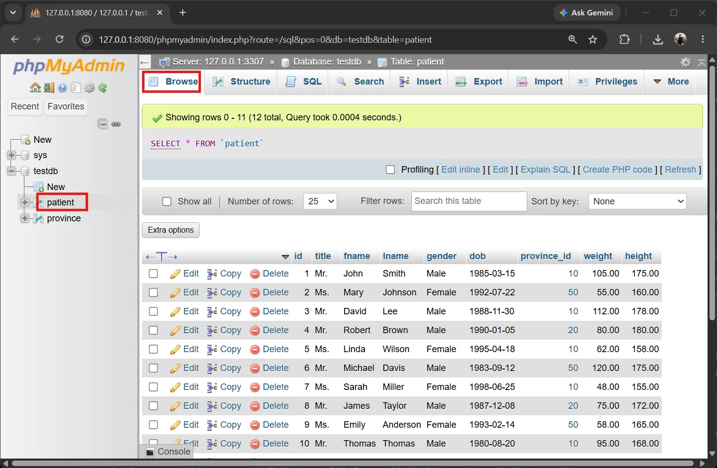
Two things to note:
- We didn’t specify the
idcolumn because it isAUTO_INCREMENT— the database counts the number for us automatically (1, 2, 3, …) province_idis given as a province code (e.g.,10), not a province name, because it is a Foreign Key that points toprovince.code- Text must be enclosed in quotes, e.g.
'John','Male', while numbers can be written directly, e.g.105.00 - Dates use the
YYYY-MM-DDformat, e.g.'1985-03-15'means March 15, 1985
6. SELECT — retrieve data#
Now we’ve reached the heart of the article. SELECT is the most frequently used command, because most of the time we want to “look at” data rather than change it. It’s like asking the database “What data do you have? Show me.”
6.1 Basic format#
SELECT column1, column2, ...   -- which columns do you want to see?
FROM table_name                -- from which table?
WHERE condition; -- (optional) only rows that match the conditionNotice the command reads almost like plain English: “SELECT these columns FROM this table WHERE (some condition) …“
6.2 Test it in phpMyAdmin#
Let’s run it for real:
- Select the
testdbdatabase in the left panel, then click thepatienttable - Click the SQL tab at the top to open the command box
- Type this command:
SELECT * FROM patient;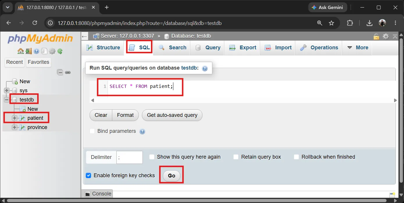
- Click the Go button in the bottom-right corner to run it
Command explanation:
SELECT— says “I want to retrieve data”*(asterisk) — means “every column” (like the multiplication sign in math, but in SQL when it follows SELECT it means “all”)FROM patient— retrieve from thepatienttable
The result is all 12 patients, every column:
Result:
| id | title | fname | lname | gender | dob | province_id | weight | height |
|---|---|---|---|---|---|---|---|---|
| 1 | Mr. | John | Smith | Male | 1985-03-15 | 10 | 105.00 | 175.00 |
| 2 | Ms. | Mary | Johnson | Female | 1992-07-22 | 50 | 55.00 | 160.00 |
| 3 | Mr. | David | Lee | Male | 1988-11-30 | 10 | 112.00 | 178.00 |
| 4 | Mr. | Robert | Brown | Male | 1990-01-05 | 20 | 80.00 | 180.00 |
| 5 | Ms. | Linda | Wilson | Female | 1995-04-18 | 10 | 62.00 | 158.00 |
| 6 | Mr. | Michael | Davis | Male | 1983-09-12 | 50 | 120.00 | 175.00 |
| 7 | Ms. | Sarah | Miller | Female | 1998-06-25 | 10 | 48.00 | 155.00 |
| 8 | Mr. | James | Taylor | Male | 1987-12-08 | 20 | 75.00 | 172.00 |
| 9 | Ms. | Emily | Anderson | Female | 1993-02-14 | 50 | 58.00 | 165.00 |
| 10 | Mr. | Thomas | Thomas | Male | 1980-08-20 | 10 | 95.00 | 168.00 |
| 11 | Ms. | Jessica | Jackson | Female | 1996-10-03 | 10 | 70.00 | 170.00 |
| 12 | Mr. | Charles | White | Male | 1982-05-17 | 50 | 88.00 | 185.00 |
6.3 Select only the columns you want#
If you don’t want to see every column, list the column names you want instead of *, separated by commas.
Select one column:
SELECT fname FROM patient;SELECT fname returns only the first-name column:
Result:
| fname |
|---|
| John |
| Mary |
| David |
| Robert |
| Linda |
| Michael |
| Sarah |
| James |
| Emily |
| Thomas |
| Jessica |
| Charles |
Select multiple columns:
SELECT fname, lname, dob FROM patient;Listing three column names separated by commas gives just those three columns:
Result:
| fname | lname | dob |
|---|---|---|
| John | Smith | 1985-03-15 |
| Mary | Johnson | 1992-07-22 |
| David | Lee | 1988-11-30 |
| Robert | Brown | 1990-01-05 |
| Linda | Wilson | 1995-04-18 |
| Michael | Davis | 1983-09-12 |
| Sarah | Miller | 1998-06-25 |
| James | Taylor | 1987-12-08 |
| Emily | Anderson | 1993-02-14 |
| Thomas | Thomas | 1980-08-20 |
| Jessica | Jackson | 1996-10-03 |
| Charles | White | 1982-05-17 |
Select all columns:
SELECT * FROM patient;SELECT * gives the same result as the full table above (every row and every column, 12 records in total).
Why not just use
*all the time? Because in real work a table can have dozens of columns — retrieving all of them is slow and messy. Selecting only the columns you actually use is faster and easier to read, and this matters even more when the query feeds a real application.
🧩 Exercise 6.1: Write a
SELECTthat shows only thefname,gender, andweightcolumns of every patient
7. WHERE — filter data by condition#
WHERE is used to filter so that only the rows that match the condition we set are shown. It’s like searching through a phone book and saying “Only show me people in Bangkok” — everyone else gets filtered out.
First, let’s look at the comparison operators used in WHERE:
| Operator | Meaning | Example |
|---|---|---|
= | equal to | gender = 'Male' |
<> or != | not equal to | gender <> 'Female' |
> | greater than | weight > 100 |
< | less than | height < 160 |
>= | greater than or equal to | weight >= 100 |
<= | less than or equal to | height <= 165 |
7.1 A single condition#
SELECT fname, lname, weight
FROM patient
WHERE weight > 100;This reads as: “Select first name, last name, and weight from the patient table, but only for people whose weight is greater than 100.” The result keeps only the people weighing 105, 112, and 120 kg; those at 100 or less are removed.
Result:
| fname | lname | weight |
|---|---|---|
| John | Smith | 105.00 |
| David | Lee | 112.00 |
| Michael | Davis | 120.00 |
7.2 Comparing dates#
WHERE also works on date columns (DATE), compared against a date in the YYYY-MM-DD format (which must be in quotes). For example, find patients born before 1990:
SELECT fname, lname, dob
FROM patient
WHERE dob < '1990-01-01';The result keeps only people born before 1990-01-01: John, David, Michael, James, Charles, and Thomas. Those born in 1990 or later are removed.
Result:
| fname | lname | dob |
|---|---|---|
| John | Smith | 1985-03-15 |
| David | Lee | 1988-11-30 |
| Michael | Davis | 1983-09-12 |
| James | Taylor | 1987-12-08 |
| Thomas | Thomas | 1980-08-20 |
| Charles | White | 1982-05-17 |
7.3 Multiple conditions with AND / OR#
We can combine multiple conditions with AND and OR:
AND— both conditions must be true (like saying “must be A and B at the same time”)OR— it’s enough for at least one condition to be true (like saying “A or B, either one”)
An AND example — find people whose weight > 100 and height < 180 (both must hold):
SELECT fname, lname, weight, height
FROM patient
WHERE weight > 100 AND height < 180;Result:
| fname | lname | weight | height |
|---|---|---|---|
| John | Smith | 105.00 | 175.00 |
| David | Lee | 112.00 | 178.00 |
| Michael | Davis | 120.00 | 175.00 |
Another AND example — find males whose weight is greater than 80:
SELECT *
FROM patient
WHERE gender = 'Male' AND weight > 80;Result:
| id | title | fname | lname | gender | dob | province_id | weight | height |
|---|---|---|---|---|---|---|---|---|
| 1 | Mr. | John | Smith | Male | 1985-03-15 | 10 | 105.00 | 175.00 |
| 3 | Mr. | David | Lee | Male | 1988-11-30 | 10 | 112.00 | 178.00 |
| 6 | Mr. | Michael | Davis | Male | 1983-09-12 | 50 | 120.00 | 175.00 |
| 10 | Mr. | Thomas | Thomas | Male | 1980-08-20 | 10 | 95.00 | 168.00 |
| 12 | Mr. | Charles | White | Male | 1982-05-17 | 50 | 88.00 | 185.00 |
An OR example — find “all males” or “anyone whose weight is over 100” (anyone matching either condition is shown):
SELECT *
FROM patient
WHERE gender = 'Male' OR weight > 100;Result (all males — since no female already weighs over 100):
| id | title | fname | lname | gender | dob | province_id | weight | height |
|---|---|---|---|---|---|---|---|---|
| 1 | Mr. | John | Smith | Male | 1985-03-15 | 10 | 105.00 | 175.00 |
| 3 | Mr. | David | Lee | Male | 1988-11-30 | 10 | 112.00 | 178.00 |
| 4 | Mr. | Robert | Brown | Male | 1990-01-05 | 20 | 80.00 | 180.00 |
| 6 | Mr. | Michael | Davis | Male | 1983-09-12 | 50 | 120.00 | 175.00 |
| 8 | Mr. | James | Taylor | Male | 1987-12-08 | 20 | 75.00 | 172.00 |
| 10 | Mr. | Thomas | Thomas | Male | 1980-08-20 | 10 | 95.00 | 168.00 |
| 12 | Mr. | Charles | White | Male | 1982-05-17 | 50 | 88.00 | 185.00 |
Common beginner mistakes:
- Text must be wrapped in quotes, e.g.
gender = 'Male'(forgetting this errors)- Numbers do not take quotes, e.g.
weight > 100- Dates must use the
YYYY-MM-DDformat and must be in quotes, e.g.'1990-01-01'
🧩 Exercise 7.1: Write a query to find patients in Bangkok province (
province_id = 10), showing their first and last name
8. ORDER BY — sort the results#
Normally, the rows returned by SELECT may appear in an unpredictable order. ORDER BY lets us sort the data by a column of our choice. It’s like organizing a student list by class number, or ranking exam scores from highest to lowest.
8.1 Basic format#
SELECT column1, column2, ...
FROM table_name
ORDER BY column1 ASC|DESC;ASC(Ascending) — low to high / A to Z (if omitted,ASCis the default)DESC(Descending) — high to low / Z to A
8.2 Example: sort by weight, high to low#
SELECT fname, lname, weight, height
FROM patient
WHERE weight > 100 AND height < 180
ORDER BY weight DESC;This query first filters for people with weight > 100 and height < 180, then sorts them by weight from high to low (DESC). The heaviest person appears at the top:
Result (sorted by weight, high to low):
| fname | lname | weight | height |
|---|---|---|---|
| Michael | Davis | 120.00 | 175.00 |
| David | Lee | 112.00 | 178.00 |
| John | Smith | 105.00 | 175.00 |
8.3 Example: sort by date of birth (age)#
SELECT fname, lname, dob
FROM patient
ORDER BY dob DESC;A note on dates: A “larger” date value means a “later” date (newer = younger). So
ORDER BY dob DESC(high to low) sorts from youngest to oldest — the youngest person is at the top. If you want oldest to youngest, switch toORDER BY dob ASC
Result (newest birth date / youngest at the top):
| fname | lname | dob |
|---|---|---|
| Sarah | Miller | 1998-06-25 |
| Jessica | Jackson | 1996-10-03 |
| Linda | Wilson | 1995-04-18 |
| Emily | Anderson | 1993-02-14 |
| Mary | Johnson | 1992-07-22 |
| Robert | Brown | 1990-01-05 |
| David | Lee | 1988-11-30 |
| James | Taylor | 1987-12-08 |
| John | Smith | 1985-03-15 |
| Michael | Davis | 1983-09-12 |
| Charles | White | 1982-05-17 |
| Thomas | Thomas | 1980-08-20 |
8.4 Sorting by multiple columns#
We can sort by more than one column, specified as a hierarchy — sort by the first column first, then within each group sort by the second column.
SELECT fname, lname, gender, weight
FROM patient
ORDER BY gender ASC, weight DESC;This command says: sort by gender from A to Z first (Female before Male), then within each gender, sort by weight from high to low:
Result (gender A→Z, then weight high→low within each gender):
| fname | lname | gender | weight |
|---|---|---|---|
| Jessica | Jackson | Female | 70.00 |
| Linda | Wilson | Female | 62.00 |
| Emily | Anderson | Female | 58.00 |
| Mary | Johnson | Female | 55.00 |
| Sarah | Miller | Female | 48.00 |
| Michael | Davis | Male | 120.00 |
| David | Lee | Male | 112.00 |
| John | Smith | Male | 105.00 |
| Thomas | Thomas | Male | 95.00 |
| Charles | White | Male | 88.00 |
| Robert | Brown | Male | 80.00 |
| James | Taylor | Male | 75.00 |
Sorting by multiple columns is very useful for reports — e.g., you want to see students grouped by class, then within each class ranked by exam score.
🧩 Exercise 8.1: Sort patients by height from high to low, showing first name and height
9. Calculating in a query — calculated columns#
Besides retrieving existing columns, SQL can compute new values on the fly using the math operators + - * /, and name the resulting column with AS. It’s like entering a “formula” in Excel that calculates a new value from existing columns.
The computed result is called a calculated column — it is not actually stored in the table; it only exists at the moment the query runs.
9.1 Example: calculate each patient’s BMI#
BMI (Body Mass Index) is calculated with the formula weight(kg) / (height in meters)². The problem is that our table stores height in centimeters (e.g., 175), so we have to divide by 100 to get meters (1.75) first.
SELECT fname,
       lname,
       weight,
       height,
       weight / ((height / 100) * (height / 100)) AS BMI
FROM patient;Explaining the formula layer by layer:
height / 100— convert centimeters to meters (e.g., 175 → 1.75)(height / 100) * (height / 100)— height in meters, squared (m²)weight / (...)— divide weight by m² to get BMIAS BMI— name this resulting columnBMI(if you don’t name it, the long formula shows up as the column header, which looks ugly)
Result:
| fname | lname | weight | height | BMI |
|---|---|---|---|---|
| John | Smith | 105.00 | 175.00 | 34.29 |
| Mary | Johnson | 55.00 | 160.00 | 21.48 |
| David | Lee | 112.00 | 178.00 | 35.35 |
| Robert | Brown | 80.00 | 180.00 | 24.69 |
| Linda | Wilson | 62.00 | 158.00 | 24.84 |
| Michael | Davis | 120.00 | 175.00 | 39.18 |
| Sarah | Miller | 48.00 | 155.00 | 19.98 |
| James | Taylor | 75.00 | 172.00 | 25.35 |
| Emily | Anderson | 58.00 | 165.00 | 21.30 |
| Thomas | Thomas | 95.00 | 168.00 | 33.66 |
| Jessica | Jackson | 70.00 | 170.00 | 24.22 |
| Charles | White | 88.00 | 185.00 | 25.71 |
Why not store a BMI column in the table? Because if you did, every time the weight changes you’d have to update BMI yourself — forget once and the data is inconsistent. Calculating it in the query like this saves space and removes any chance of mismatched data.
Up next: We’ll take this calculated BMI and use it with
GROUP BYto find the average BMI by gender (next section)
🧩 Exercise 9.1: Show each patient’s weight in pounds (kg × 2.20462), naming the resulting column
weight_lbs
10. GROUP BY — group and summarize data#
GROUP BY is used to group rows that share the same value together, then summarize each group with special functions. It’s like a teacher splitting students by class and then counting how many are in each class, or finding each class’s average score.
Here are the commonly used summary functions (called aggregate functions):
| Function | What it does | Example |
|---|---|---|
COUNT() | Count the number of rows | how many patients |
SUM() | Total sum | total weight |
AVG() | Average | average weight |
MAX() | Largest value | maximum weight |
MIN() | Smallest value | minimum weight |
10.1 Basic format#
SELECT column1, aggregate_function(column2)
FROM table_name
GROUP BY column1;10.2 Example: find the average weight and height by gender#
SELECT gender, AVG(weight), AVG(height)
FROM patient
GROUP BY gender;The database will split the patients into groups by gender (Male / Female), then compute AVG() for each group separately. The result is one summary row per gender:
Result:
| gender | AVG(weight) | AVG(height) |
|---|---|---|
| Male | 96.43 | 176.14 |
| Female | 58.60 | 161.60 |
Reading the result: the 7 males have an average weight of 96.43 kg and average height of 176.14 cm, while the 5 females have an average weight of 58.60 kg and average height of 161.60 cm.
10.3 Other aggregate functions#
Let’s swap the summary function — all four of these commands give two rows (Male and Female) as before, but with different summaries.
COUNT(*) — count the number of patients in each gender:
SELECT gender, COUNT(*) FROM patient GROUP BY gender;Result:
| gender | COUNT(*) |
|---|---|
| Male | 7 |
| Female | 5 |
SUM(weight) — total weight in each gender:
SELECT gender, SUM(weight) FROM patient GROUP BY gender;Result:
| gender | SUM(weight) |
|---|---|
| Male | 675.00 |
| Female | 293.00 |
MAX(weight) — maximum weight in each gender:
SELECT gender, MAX(weight) FROM patient GROUP BY gender;Result:
| gender | MAX(weight) |
|---|---|
| Male | 120.00 |
| Female | 70.00 |
MIN(weight) — minimum weight in each gender:
SELECT gender, MIN(weight) FROM patient GROUP BY gender;Result:
| gender | MIN(weight) |
|---|---|
| Male | 75.00 |
| Female | 48.00 |
10.4 Calculate before summarizing: find the average BMI by gender#
We can take the BMI formula (from the previous section) and wrap it inside AVG() directly, to find the average BMI of each gender.
SELECT gender,
       AVG(weight / ((height / 100) * (height / 100))) AS BMI
FROM patient
GROUP BY gender;You can picture the steps like this:
- SQL first computes the BMI for every patient (from
weightandheight) - It splits the people into groups by gender
AVG()finds the average BMI of each groupAS BMInames the resulting columnBMI
Result:
| gender | BMI |
|---|---|
| Male | 31.18 |
| Female | 22.37 |
Males have a higher average BMI than females (consistent with their higher average weight).
10.5 Using it with dates: find the oldest and youngest in each gender#
MIN() and MAX() also work on dates. For example, find the oldest (earliest) and newest (latest) birth dates among patients in each gender:
SELECT gender,
       MIN(dob) AS oldest,
       MAX(dob) AS youngest
FROM patient
GROUP BY gender;Result:
| gender | oldest | youngest |
|---|---|---|
| Male | 1980-08-20 | 1990-01-05 |
| Female | 1992-07-22 | 1998-06-25 |
MIN(dob)— the oldest birth date (oldest person) in the group, e.g. for males it’s1980-08-20MAX(dob)— the newest birth date (youngest person) in the group, e.g. for females it’s1998-06-25
Tip: Using
ASto name the resulting columns (e.g.oldest,youngest) makes the result table much easier to read.
Real-world applications: Count patients by province, find average BMI by gender, count orders by customer, compute total sales by product category, count students by faculty
🧩 Exercise 10.1: Count the number of patients in each province, grouped by
province_id
11. JOIN — combine multiple tables together#
In a real database, data is often split across multiple tables to reduce redundancy. In our example, the patient table stores only the “province code” (province_id), while the “province name” is stored separately in the province table. When we want to see both the patient name and the province name at the same time, we use JOIN to combine the two tables.
It’s like the VLOOKUP function in Excel — you take a value from one table to “look it up” in another table in order to pull in related data for display.
11.1 LEFT JOIN#
There are several kinds of JOIN, but the most commonly used is LEFT JOIN, which returns:
- Every row from the left table (the table written after FROM)
- Plus the matching data from the right table (the table written after LEFT JOIN)
- If the right table has no matching data, the right table’s columns are
NULL(empty)
11.2 Basic format#
SELECT column1, column2, ...
FROM table1
LEFT JOIN table2
ON table1.column = table2.column;The ON line is very important — it tells the database “which column to match the two tables on.” Here, we match the patient’s province_id against the province’s code.
11.3 Example: show each patient’s province name#
SELECT patient.id,
       patient.fname,
       patient.dob,
       patient.province_id,
       province.name
FROM patient
LEFT JOIN province
ON patient.province_id = province.code;Part-by-part explanation:
FROM patient— thepatienttable is the left table (we want to see every patient)LEFT JOIN province— attach theprovincetable alongside (the right table)ON patient.province_id = province.code— match by checking which province’scodethe patient’sprovince_idcorresponds to
Result:
| id | fname | dob | province_id | name |
|---|---|---|---|---|
| 1 | John | 1985-03-15 | 10 | Bangkok |
| 2 | Mary | 1992-07-22 | 50 | Chiang Mai |
| 3 | David | 1988-11-30 | 10 | Bangkok |
| 4 | Robert | 1990-01-05 | 20 | Nakhon Ratchasima |
| 5 | Linda | 1995-04-18 | 10 | Bangkok |
| 6 | Michael | 1983-09-12 | 50 | Chiang Mai |
| 7 | Sarah | 1998-06-25 | 10 | Bangkok |
| 8 | James | 1987-12-08 | 20 | Nakhon Ratchasima |
| 9 | Emily | 1993-02-14 | 50 | Chiang Mai |
| 10 | Thomas | 1980-08-20 | 10 | Bangkok |
| 11 | Jessica | 1996-10-03 | 10 | Bangkok |
| 12 | Charles | 1982-05-17 | 50 | Chiang Mai |
Notice the last column, name — the patient table didn’t originally have this column, but by joining with the province table we can pull in the province name, e.g. province_id 10 → Bangkok, 50 → Chiang Mai.
What if a province isn’t in the
provincetable? The patient is still shown (because it’s a LEFT JOIN, the left table is kept in full), but the province-name column will beNULL.
11.4 Use a table alias to make the query shorter and easier to read#
Notice above that we had to type patient.id, patient.fname … over and over, getting long. SQL lets us give a table a short name (table alias) so we can type less.
SELECT p.id,
       p.fname,
       p.dob,
       p.province_id,
       pr.name
FROM patient p
LEFT JOIN province pr
ON p.province_id = pr.code;patient p— give thepatienttable the aliaspprovince pr— give theprovincetable the aliaspr
Now you can write p.id instead of patient.id. The result is exactly the same (the same 12 rows) — an alias is just a nickname; it doesn’t change the result, but it makes the query much shorter and easier to read, especially when joining several tables.
🧩 Exercise 11.1: Write a query that shows patient names and province names, using the table aliases
pforpatientandprforprovince
12. INSERT — add data#
We actually already used INSERT in section 5 (when adding sample data). This time let’s look at the format in more detail. INSERT is used to add a new row to a table — different from UPDATE (modify existing data) and DELETE (remove data).
12.1 Basic format#
INSERT INTO table_name (column1, column2, ...)
VALUES (value1, value2, ...);- The number of values must match the number of columns, and the order must line up
- Text must be enclosed in quotes, e.g.
'Somchai', while numbers can be written directly, e.g.78.00
12.2 Add a single row#
Add one new patient:
INSERT INTO patient (title, fname, lname, gender, dob, province_id, weight, height)
VALUES ('Mr.', 'Somchai', 'Jaidee', 'Male', '1990-01-01', 10, 78.00, 175.00);You don’t need to specify id because it is AUTO_INCREMENT — the database counts it for you (the next patient will get id = 13). And province_id = 10 means Bangkok, which must be a code that exists in the province table.
12.3 Add multiple rows#
If you want to add several people, you don’t need a separate INSERT per row — just separate each set of values with a comma (like we did in section 5):
INSERT INTO patient (title, fname, lname, gender, dob, province_id, weight, height) VALUES
  ('Ms.', 'Naree', 'Phromma',  'Female', '1995-05-20', 30, 52.00, 162.00),
('Ms.', 'Ploy', 'Srisuwan', 'Female', '1997-03-10', 30, 50.00, 160.00);A single command adds two people at once: Naree (id=14) and Ploy (id=15).
Note: We set
province_id = 30(Nakhon Pathom) for Naree and Ploy because in the original sample data no patient lives in province 30 at all. This lets the upcomingUPDATEandDELETEsections useWHERE province_id = 30to target just these newly-added people conveniently, without affecting the original 12.
Tip: Adding multiple rows in a single command (a multiple-row INSERT) is faster than running
INSERTonce per row, especially when loading large amounts of data.
🧩 Exercise 12.1: Add one new patient using your own data (remember that
province_idmust be acodethat exists in theprovincetable)
13. UPDATE — modify data#
UPDATE is used to modify existing data in a table — different from INSERT, which adds new rows. UPDATE is like using correction fluid to fix data in a ledger — it doesn’t add a new page; it edits what’s already written.
13.1 Basic format#
UPDATE table_name
SET column1 = value1,
    column2 = value2
WHERE condition;UPDATE table_name— says which table to modifySET column = new_value— assigns a new value to a column (separate multiple columns with commas)WHERE condition— selects which rows to modify (very important! explained below)
13.2 Modify a single row#
Example: change the weight of the patient Somchai (id = 13 — the person we just added in the INSERT section) from 78.00 to 80.00:
UPDATE patient
SET weight = 80
WHERE id = 13;This reads as: “Update the patient table, set weight to 80, for only the row where id = 13.” As a result, Somchai’s weight changes:
Before:
| id | fname | weight |
|---|---|---|
| 13 | Somchai | 78.00 |
After:
| id | fname | weight |
|---|---|---|
| 13 | Somchai | 80.00 |
Tip: After editing, we usually run
SELECT * FROM patient WHERE id = 13;to verify the data actually changed, becauseUPDATEdoesn’t return a result table to look at.
13.3 Modify multiple columns at once#
If you want to change both weight and height in one command, separate each column = value with a comma:
UPDATE patient
SET weight = 80,
    height = 180
WHERE id = 13;Now Somchai will have a weight of 80 and a height of 180 at the same time.
13.4 Modify multiple rows#
If the WHERE condition matches multiple rows, UPDATE will modify every matching row. Example: set the weight of the patients we just added (Naree and Ploy, who are at province_id = 30) to 60.00:
UPDATE patient
SET weight = 60
WHERE province_id = 30;This command modifies every row where province_id = 30, which is 2 people (Naree id=14 and Ploy id=15):
Before:
| id | fname | weight |
|---|---|---|
| 14 | Naree | 52.00 |
| 15 | Ploy | 50.00 |
After:
| id | fname | weight |
|---|---|---|
| 14 | Naree | 60.00 |
| 15 | Ploy | 60.00 |
⚠️ Important warning: If you forget the
WHERE, the database will modify every row in the table!sqlUPDATE patient SET weight = 80; -- everyone instantly gets a weight of 80That’s usually not what you intended. Always check the
WHEREbefore runningUPDATE.
🧩 Exercise 13.1: Change patient Somchai’s (
id = 13) height from 175.00 to 178.00
14. DELETE — remove data#
DELETE is used to permanently remove rows from a table — different from UPDATE, which only edits data. DELETE means “throw it away,” so use it with care: once data is deleted, it is hard to recover.
14.1 Basic format#
DELETE FROM table_name
WHERE condition;Notice that DELETE has no column names — because it deletes the whole row, not individual columns.
14.2 Delete a single row#
Example: remove the patient Somchai (id = 13 — the person we just added) from the table:
DELETE FROM patient
WHERE id = 13;After running, Somchai’s row disappears from the patient table. All other rows remain intact.
14.3 Delete multiple rows#
If WHERE matches multiple rows, all of them are deleted. Example: delete the patients we just added (Naree and Ploy, who are at province_id = 30):
DELETE FROM patient
WHERE province_id = 30;This command deletes 2 rows — Naree (id=14) and Ploy (id=15) — the patients we just added in the INSERT section.
⚠️ Important warning: If you forget the
WHERE, you will delete every row in the table!sqlDELETE FROM patient; -- delete every row! The table structure stays, but the data is goneAlways check the
WHEREbefore runningDELETE.
Note: After
DELETEthe table still exists (the column structure is not removed) — only the data inside is deleted. If you want to remove the entire table — structure plus data — useDROP TABLE patient;, but that’s rarely used and dangerous; use it with great care.
🧩 Exercise 14.1: Try adding one new patient (with
INSERT) and then deleting it withDELETE— notice that after deletion, that row is gone.
15. Summary#
Congratulations! You have learned the SELECT command and all its components for retrieving and shaping results. Let’s review:
SELECT— choose which columns to show (SELECT *means every column)WHERE— filter for only rows that match a condition, supportingAND/ORand comparisons on both numbers and datesORDER BY— sort the results (ASClow to high /DESChigh to low), with support for multiple columns- Calculated columns — compute new values in the query with
+ - * /and name them withAS(e.g., BMI) GROUP BY— group rows and summarize them with aggregate functions (COUNT,SUM,AVG,MIN,MAX)JOIN— combine multiple tables together, e.g.LEFT JOIN, using table aliases to keep it shortINSERT— add new rows to a table, one at a time or several in a single commandUPDATE— modify existing data, single or multiple rows (don’t forgetWHERE, or every row is modified)DELETE— permanently remove rows from a table (don’t forgetWHERE, or every row is deleted)
Think of these commands as “sentences” you use to ask the database questions:
“SELECT first name and weight FROM the patient table, for only (WHERE) people whose weight is over 100, then sort (ORDER BY) from high to low.”
Once you understand SELECT and these components, you can retrieve and analyze data from a database efficiently, and build on this foundation for reporting, analytics, and building applications that connect to a database.