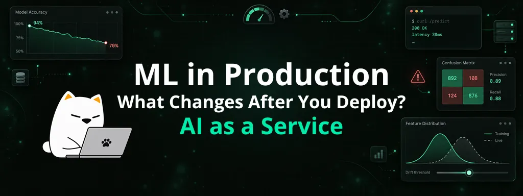
ML in Production — What Changes After You Deploy
Life after deploy — the exam never ends, overfitting vs leakage, data and concept drift, model decay, and picking metrics that match the money
The previous part set up the tools and revisited the ML basics that matter for production — three datasets, a baseline, and the three silent-bug terms: Model Artifact, Feature Schema, and Preprocessor.
This part turns to what actually changes once a model leaves the notebook and starts serving real users.
Setting Up#
Every example below runs in a Jupyter notebook, in the same ml-refresher folder from the previous part. If you already set up that environment in Part 2 — ML Refresher ↗, skip the rest of this section — just reactivate it and read on.
First, make sure Python 3 is installed. Grab the latest from python.org/downloads ↗ — on Windows tick “Add python.exe to PATH” during install; on Linux (Ubuntu) run sudo apt update && sudo apt install python3. Verify with:
python --version # use python3 on Linux; on Windows try py --version if python failsThen reactivate the environment (or create it fresh below):
Windows (PowerShell):
cd ml-refresher
.venv\Scripts\activatemacOS / Linux:
cd ml-refresher
source .venv/bin/activateStarting fresh? Create the environment and install everything in one go (use python3 on Linux):
mkdir ml-refresher
cd ml-refresher
python -m venv .venv        # then activate it with the command above
pip install notebook pandas numpy scikit-learn matplotlib joblibThen launch the notebook and you are ready:
jupyter notebook1. What Changes When a Model Goes to Production#
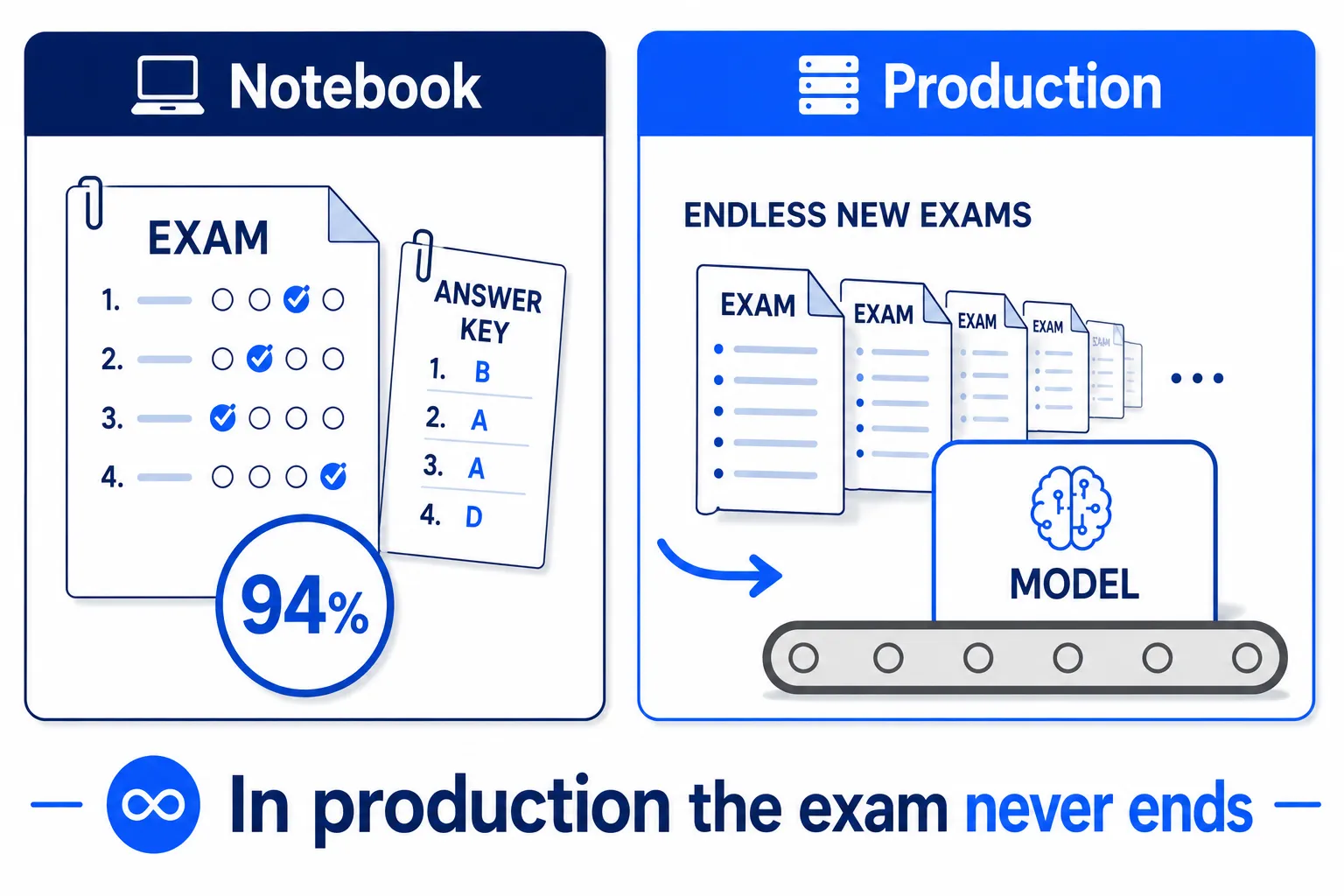
In class, model evaluation is fairly straightforward.
Split the data into a Training Set and a Test Set, train on the training set, then measure against data the model has never seen.
Follow along with a small spam dataset — create spam.csv in the notebook folder (the last column spam is the answer: 1 = spam, 0 = not spam):
length,num_links,num_capital_words,sender_domain_new,spam
257,3,7,1,1
645,0,0,0,0
524,1,1,0,0
280,3,7,1,1
500,0,1,0,0
430,0,0,0,1
231,4,10,1,1
384,1,0,0,0
350,0,1,0,0
179,5,10,1,1
581,0,0,0,0
389,0,1,0,0
217,4,7,1,1
526,0,2,0,0
487,0,2,0,0
205,5,7,1,1
612,0,1,0,0
363,0,1,0,0
298,4,9,1,1
515,0,1,0,0
327,1,1,0,0
183,3,6,1,1
614,0,2,0,0
333,0,1,0,0
294,4,9,1,1
551,1,2,0,0
414,0,0,0,0
293,3,9,1,1
457,1,2,0,0
341,0,1,0,0
212,4,6,1,1
561,1,0,0,0
339,0,2,0,0
191,3,8,1,1
561,1,1,0,0
497,0,2,0,0
281,3,9,1,1
520,0,0,0,0
552,1,1,0,0
218,4,6,1,1
432,0,2,0,0
322,1,1,0,0
195,4,8,1,1
471,1,0,0,0
600,1,0,0,0
197,5,7,1,1
415,1,1,0,0
510,1,1,0,0
233,4,9,1,1
375,1,0,0,0
602,0,1,0,0
201,4,6,1,1
429,0,2,0,0
638,1,2,0,0
288,3,10,1,1
407,0,2,0,0
384,1,2,0,0
242,4,7,1,1
581,0,2,0,0
355,1,1,0,0Then train and score it — the classroom flow, start to finish:
import pandas as pd
from sklearn.ensemble import RandomForestClassifier
from sklearn.model_selection import train_test_split

df = pd.read_csv("spam.csv")
X = df.drop(columns="spam")   # the features the model sees
y = df["spam"]                # the answer to learn

X_train, X_test, y_train, y_test = train_test_split(
    X, y, test_size=0.2, random_state=42
)

model = RandomForestClassifier(random_state=42).fit(X_train, y_train)
print(round(model.score(X_test, y_test), 2)) # one number on unseen data → 0.92In the end one number comes out, e.g.:
Accuracy = 92%
Looks easy — 92% counts as good, job done.
But once the model goes to production, everything changes, because the Test Set is no longer a single set.
New data flows at the model every day, and it never stops.
Every request from a real user is a new exam question for the model.
At least three things differ from the classroom.
1.1 The Exam Never Ends#
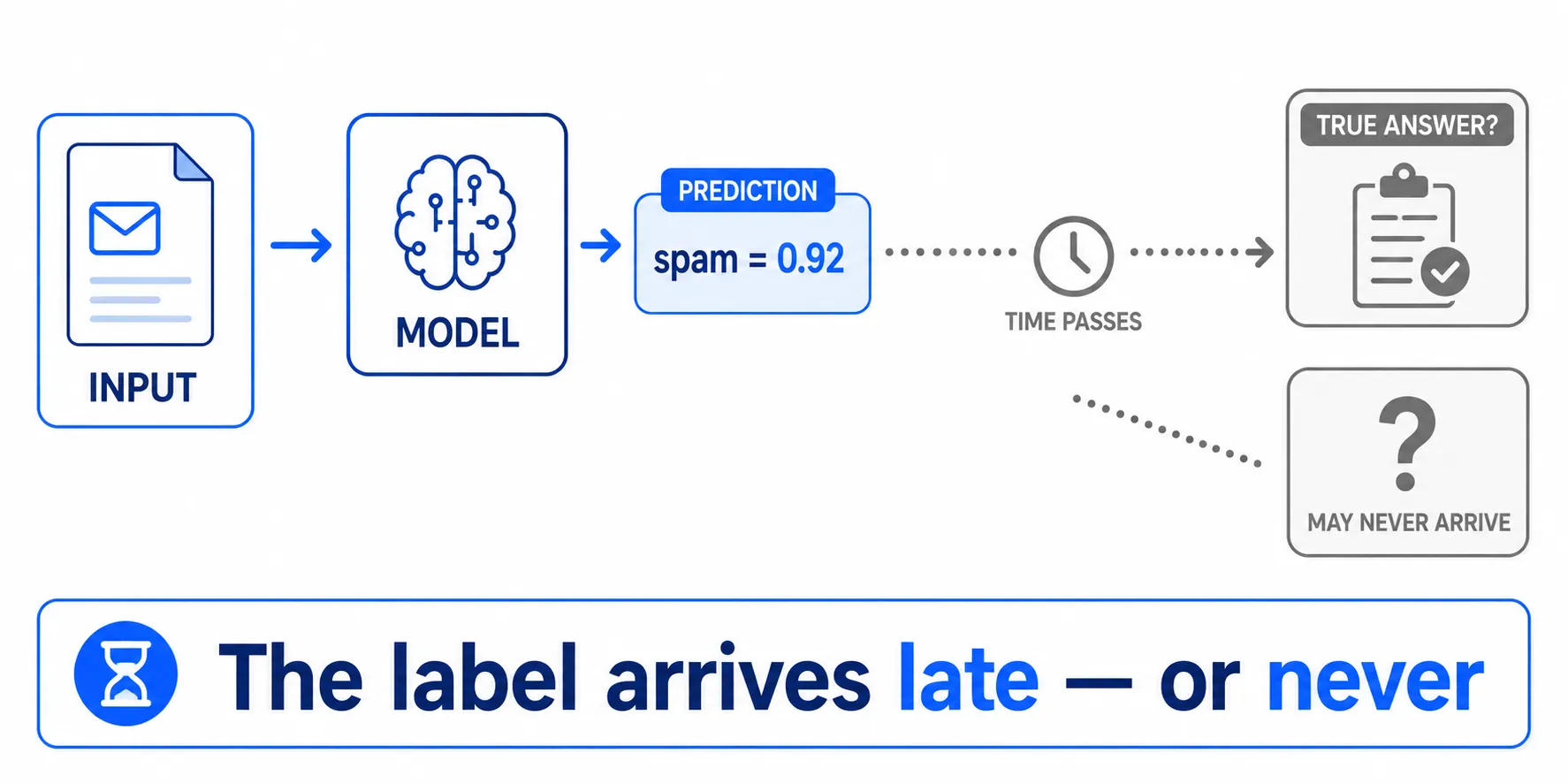
In class there is X_test — and crucially, there is y_test.
That means both the questions and the answer key are in hand.
If the model predicts an email is spam, opening y_test immediately shows whether that was right.
But in production there is usually only:
Input → Prediction → done
Suppose a new email arrives and the model answers:
spam = 0.92
Whether that email truly is spam may still be unknown.
The answer may arrive later — e.g. a user clicking “Not Spam” — or never arrive at all.
Measuring accuracy in production is therefore much harder than in a notebook.
During training, the answers are ready. In production, the answers may be late — or never come.
1.2 Real Data May Not Look Like Training Data#
When splitting with train_test_split(), the quiet assumption is that the Training Set and Test Set come from the same data.
So the Test Set is a fairly honest sample of what the model learned.
Production offers no such guarantee.
Suppose a spam detection model was trained on this year’s email.
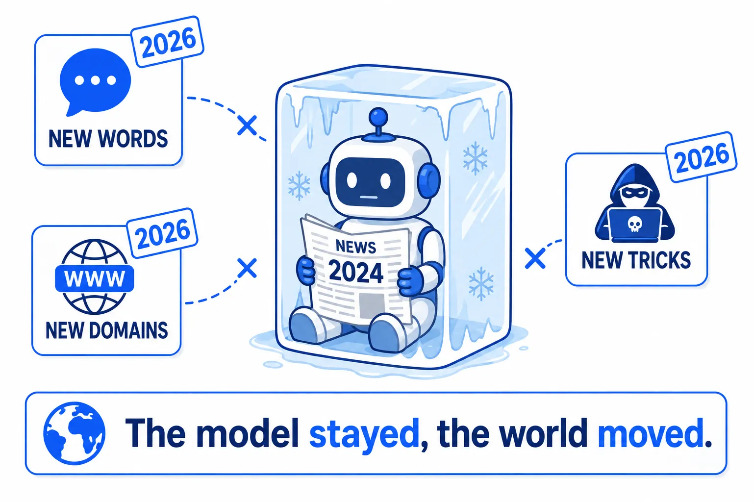
Six months later, spam has changed shape — senders use new words, new domains, new ways to evade filters.
The model is unchanged, but the world around it has already moved on.
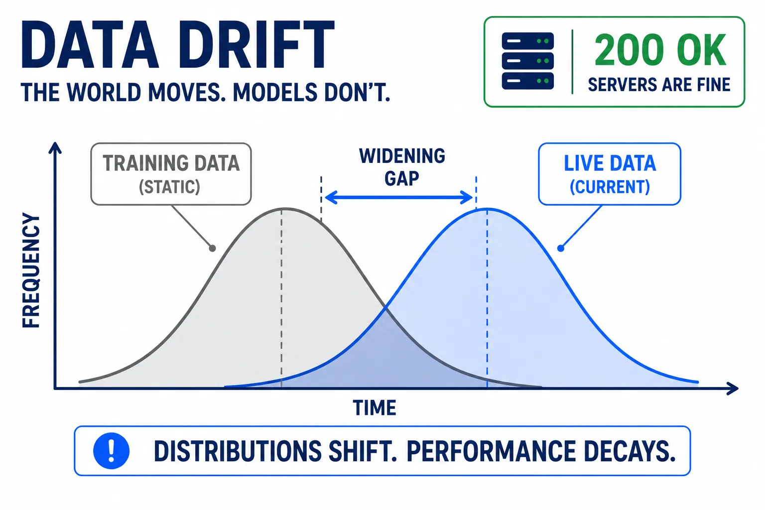
Incoming production data can drift further and further from the training data.
This is one reason a model that scored 92% at deploy can slide to 88%, 85%, or 70% while nothing on the server is broken.
The model didn’t change — the data did.
And that is why monitoring must cover not only the server but also the data flowing into the model.
1.3 Accuracy Alone Is Not Enough — Latency Matters Too#
In a notebook, the usual question is:
“Which model is most accurate?”
Production adds another:
“And is it fast enough?”
Because model.predict() no longer runs in a notebook — it runs inside an API request handler.
The real flow is:
User → API → Model Predict → Response → User
If the model takes 20 milliseconds, users barely notice.
But if a prediction takes 5 seconds, every request waits 5 seconds.
And when many users arrive at once, the problem compounds.
So the highest-accuracy model is not automatically the best model for production.
Sometimes a little accuracy is traded away for a faster model that uses less memory and handles more requests.
This is the new trade-off once a model leaves the notebook:
Prediction Quality ↔ Latency ↔ Cost
A good production model is therefore not just one that predicts accurately.
It must also be fast enough, stable enough, and affordable.
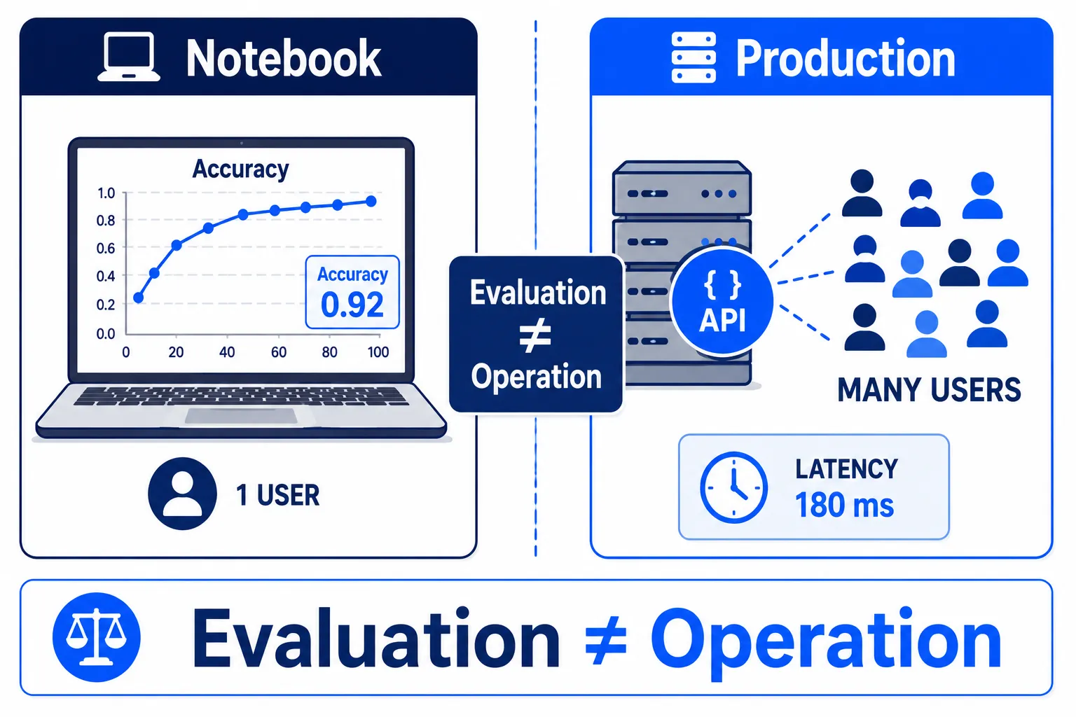
This is the key difference between evaluating a model and operating a model.
In class, the story may end with one number:
Accuracy = 92%
In production, the questions keep coming:
Is the model still accurate right now? Does incoming data still look the same? Is it answering fast enough? Can it hold the request volume? And do we even know whether the answers it gave were correct?
Because in production the exam never runs out, and the model never truly finishes the test.
Two more classic Machine Learning problems need a refresher before production: Overfitting and Data Leakage.
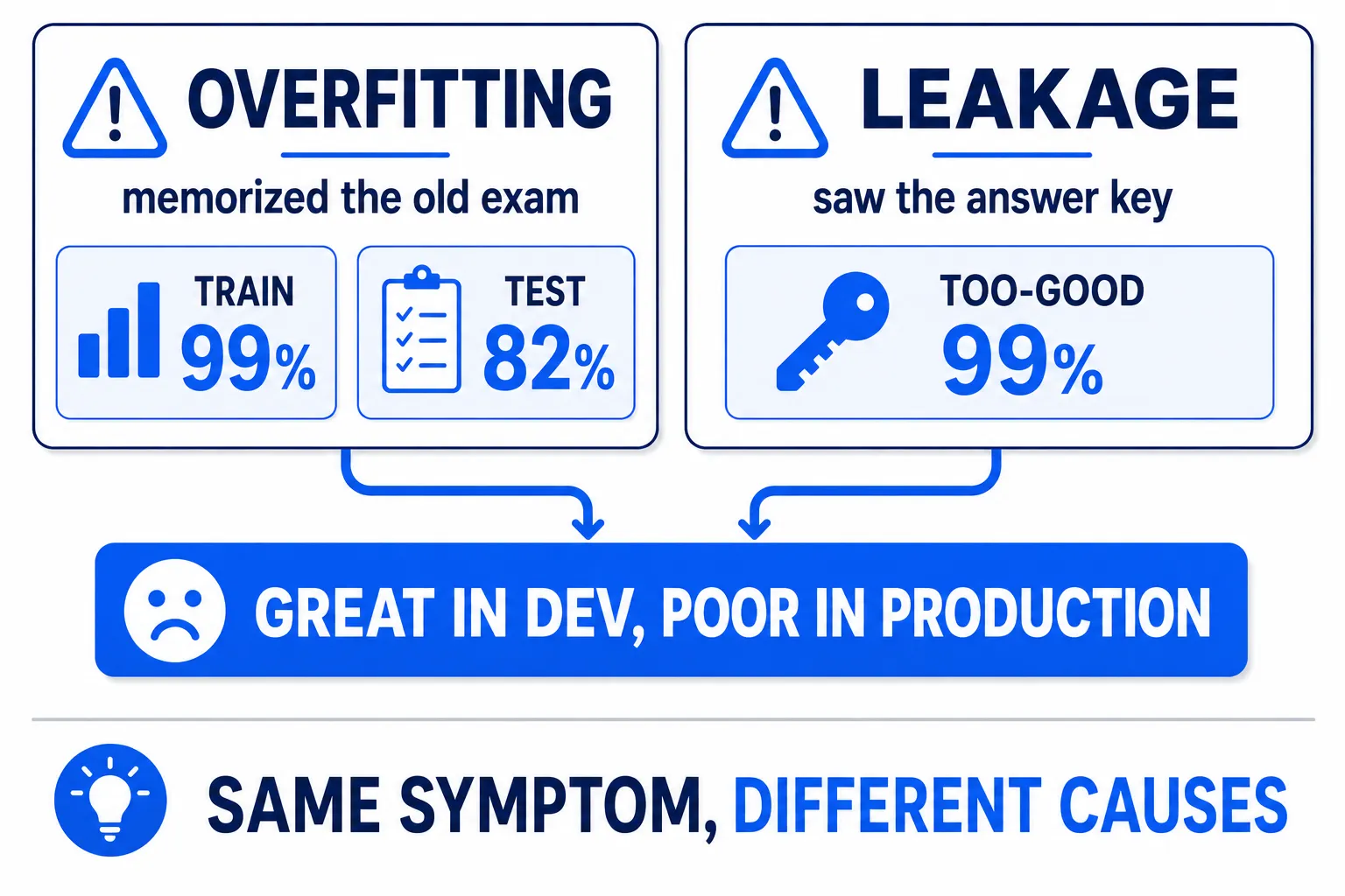
Both produce a very similar symptom:
Looks great in experiments, worse than expected in real use.
But their causes differ.
1.4 Overfitting — Memorizes Too Well to Handle Anything New#
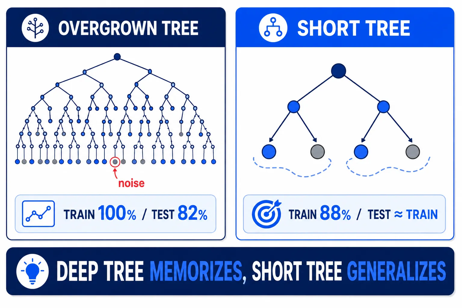
Overfitting happens when a model fails to learn a pattern that generalizes to new data, and instead memorizes too much detail of the training data.
Picture a student who never understood the material but memorized every past exam along with its answers.
If the real exam matches the old one — perfect score.
Change the questions even slightly, and it all falls apart.
Machine Learning works the same way.
The usual symptom:
Training score very high, Test score clearly lower.
For example:
Training Accuracy = 99%
Test Accuracy = 82%
See it with your own eyes using a real file — create signups.csv, predicting whether a customer will subscribe (most rows follow “more than 2 visits = subscribe,” with 2 rows breaking the pattern as noise):
age,income,visits,subscribed
26,35000,0,0
40,55000,0,0
39,50000,6,1
36,29000,0,0
23,61000,1,0
41,49000,6,1
42,56000,2,0
22,59000,6,1
37,66000,2,0
37,60000,5,1
40,36000,1,0
40,53000,0,0
42,54000,1,1
45,42000,4,1
43,41000,6,1
36,60000,2,1Try a Decision Tree with unlimited depth:
import pandas as pd
from sklearn.tree import DecisionTreeClassifier
from sklearn.model_selection import train_test_split

df = pd.read_csv("signups.csv")
X = df.drop(columns="subscribed")
y = df["subscribed"]
X_tr, X_te, y_tr, y_te = train_test_split(X, y, test_size=0.25, random_state=42)

tree = DecisionTreeClassifier()      # no depth limit → grows until every row is memorized
tree.fit(X_tr, y_tr)

print("train:", tree.score(X_tr, y_tr))   # 1.0 — every row memorized
print("test :", tree.score(X_te, y_te)) # 0.75 — clearly below trainA fully grown tree invents special rules to memorize even the noise rows, so on unseen data it guesses wrong.
Fixes come in many forms: add data, reduce model complexity, or use regularization so the model doesn’t try so hard to memorize the training data.
Try the simplest one — cap the tree depth:
simple = DecisionTreeClassifier(max_depth=2)   # force it to learn only the main pattern
simple.fit(X_tr, y_tr)

print("train:", simple.score(X_tr, y_tr))   # 0.83 — drops from 1.0
print("test :", simple.score(X_te, y_te)) # 1.0 — higher than the full tree, the gap closesPut simply:
Overfitting = too much memorizing, too little understanding of the real pattern.
1.5 Data Leakage — the Model Sneaks a Peek at the Answer Key#
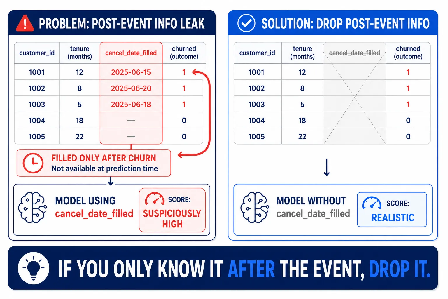
Data Leakage is sneakier, because the results can look so good that the model seems brilliant.
If leakage must be captured in one line, remember:
Data Leakage = the model got to see the answer key.
The rule is a single line:
Every feature used must be information already known at the moment a real prediction is made.
If a feature only comes into existence after the event being predicted, it must not be used as input.
A small example first — create churn.csv, predicting whether a customer will cancel the service, with a cancel_date_filled column that the system fills in only after the customer has already cancelled:
months,plan_price,support_calls,cancel_date_filled,churned
14,299,0,0,0
8,499,2,0,0
3,199,1,0,0
11,399,2,0,0
17,599,1,0,0
15,299,3,0,0
6,399,2,1,1
3,599,4,1,1
16,299,3,1,1
4,199,2,1,1
2,499,5,1,1
12,399,1,1,1Train both ways — with and without that column (same train/test split for a fair comparison):
import pandas as pd
from sklearn.ensemble import RandomForestClassifier
from sklearn.model_selection import train_test_split

df = pd.read_csv("churn.csv")
X_leaky = df.drop(columns="churned")                          # includes cancel_date_filled
X_clean = X_leaky.drop(columns="cancel_date_filled")          # drops the known-only-later column
y = df["churned"]

X_tr, X_te, y_tr, y_te = train_test_split(X_leaky, y, test_size=0.25, random_state=42)
X_tr_c = X_tr.drop(columns="cancel_date_filled")
X_te_c = X_te.drop(columns="cancel_date_filled")

leaky = RandomForestClassifier(random_state=42).fit(X_tr, y_tr)
clean = RandomForestClassifier(random_state=42).fit(X_tr_c, y_tr)

print("with leaky column :", leaky.score(X_te, y_te))    # suspiciously high
print("column dropped :", clean.score(X_te_c, y_te)) # lower — and this is the real numberOne column that is only known “afterwards” inflates the score — yet in production that column will be 0 for everyone, because at prediction time nobody has cancelled yet.
For a more dangerous version from a real hospital, continue to the next case study.
1.6 Case Study: Predicting ICU Admission#
Suppose a hospital wants a model that predicts — right when a patient is admitted — who is at risk of deteriorating badly enough to need the ICU.
The data team gathers many features from medical records:
- age
- blood pressure
- lab results
- medications received
- pre-existing conditions
And there is one more column:
icu_transfer_count
meaning the number of times the patient has been transferred to the ICU.
A miniature patients.csv for experimenting (the real one has thousands of rows):
age,blood_pressure,lab_result,icu_transfer_count,icu_admitted
68,150,1.9,2,1
61,152,2.1,0,0
72,146,2.4,3,1
66,138,1.8,0,0
65,154,2.2,1,1
69,135,2.3,0,0
70,144,1.6,2,1
63,148,1.5,0,0
67,141,2.0,3,1
62,147,1.7,0,0
71,149,1.2,1,1
64,139,2.5,0,0Train with every column, including icu_transfer_count:
import pandas as pd
from sklearn.ensemble import RandomForestClassifier
from sklearn.model_selection import train_test_split

df = pd.read_csv("patients.csv")
X = df.drop(columns="icu_admitted")
y = df["icu_admitted"]

X_tr, X_te, y_tr, y_te = train_test_split(X, y, test_size=0.25, random_state=42)
model = RandomForestClassifier(random_state=42).fit(X_tr, y_tr)
print(model.score(X_te, y_te)) # an oddly good score — be suspicious right awayThe full dataset is then used to train the model.
The result looks beautiful:
Accuracy = 99%
Everyone is delighted — the model appears to know almost exactly who will end up in the ICU.
But in reality the model may have found a simple shortcut:
if icu_transfer_count > 0
→ the patient is very likely a severe case
At a glance the model looks brilliant.
But ask the key question:
When is
icu_transfer_countfilled in?
The answer: after the patient was already transferred to the ICU.
That is the problem.
The goal is a model that predicts “will this patient need the ICU?”
But the data quietly tells it “this patient has already been in the ICU this many times.”
The model is not learning to predict the future.
It is reading a future that slipped into the training data.
The outcome came disguised as an input.
What Happens at Deploy Time?#
During training, the data was pulled from historical records.
So patients who had been in the ICU may show:
icu_transfer_count = 2
The model leans on this feature as a strong signal.
But in production the prediction is needed at admission time.
At that moment the patient has not been transferred anywhere yet.
So:
icu_transfer_count = 0
for almost everyone.
The feature that powered the 99% accuracy is nearly useless at the moment it actually matters.
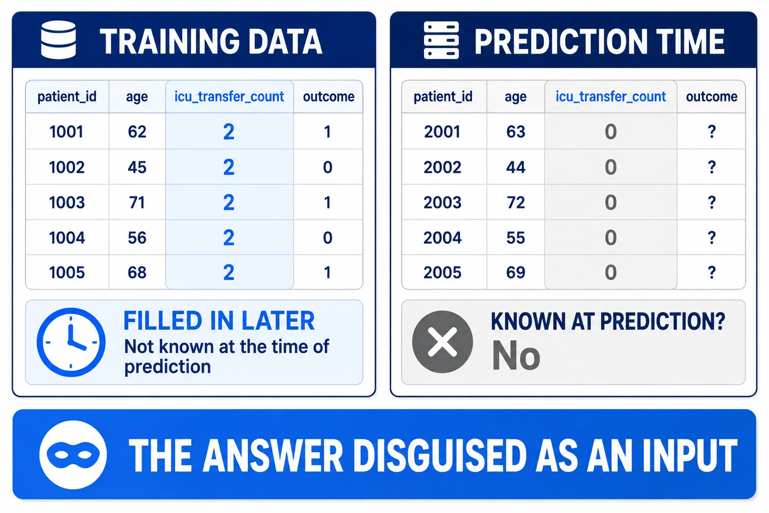
Side by side:
| At training | At real prediction | |
|---|---|---|
| Patient later admitted to the ICU | icu_transfer_count = 2 | icu_transfer_count = 0 |
| Patient never admitted to the ICU | icu_transfer_count = 0 | icu_transfer_count = 0 |
Same column name, but completely different meaning.
Training looks backward at what already happened.
Prediction stands in the present, trying to guess what has not happened yet.
That gap is exactly where Data Leakage hides.
The One Question That Catches Leakage#
Choosing features does not require a complicated checklist.
Ask every column:
“At the second the system must actually predict, is this value already known?”
If the answer is known, it may work as a feature.
- Age at admission → known
- Blood pressure at admission → known
- Lab results issued before prediction time → known
- ICU transfers after admission → not yet known
If it is not known at prediction time, the model must not see it.
1.7 How Do Overfitting and Leakage Differ?#
Both make a model look great in development and fail against the real world.
But the root causes are different:
| Overfitting | Data Leakage | |
|---|---|---|
| The problem | The model memorizes the training data | The model receives data it shouldn’t |
| Typical symptom | Training good, Test bad | Training and Test both oddly great |
| Core issue | Cannot generalize to new data | Evaluation lies that the model is good |
| Simple mental model | Memorized the old exams | Saw the answer key |
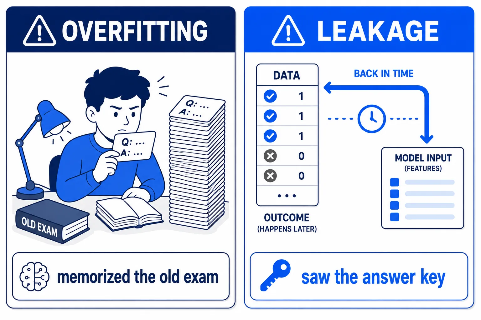
Data Leakage is among the most dangerous Machine Learning mistakes, because it does not make results look bad.
The opposite — it makes results look too good.
High accuracy. Tests pass. Beautiful charts. Everyone agrees it is ready to deploy.
Until the system meets real data.
And only then it turns out the “99% accurate” model was never actually good at predicting the future.
Before using any feature, don’t just ask “does it make the model more accurate?” Also ask “will this data actually be in hand when the system runs for real?“
1.8 Model Decay: the Reason Monitoring Exists#
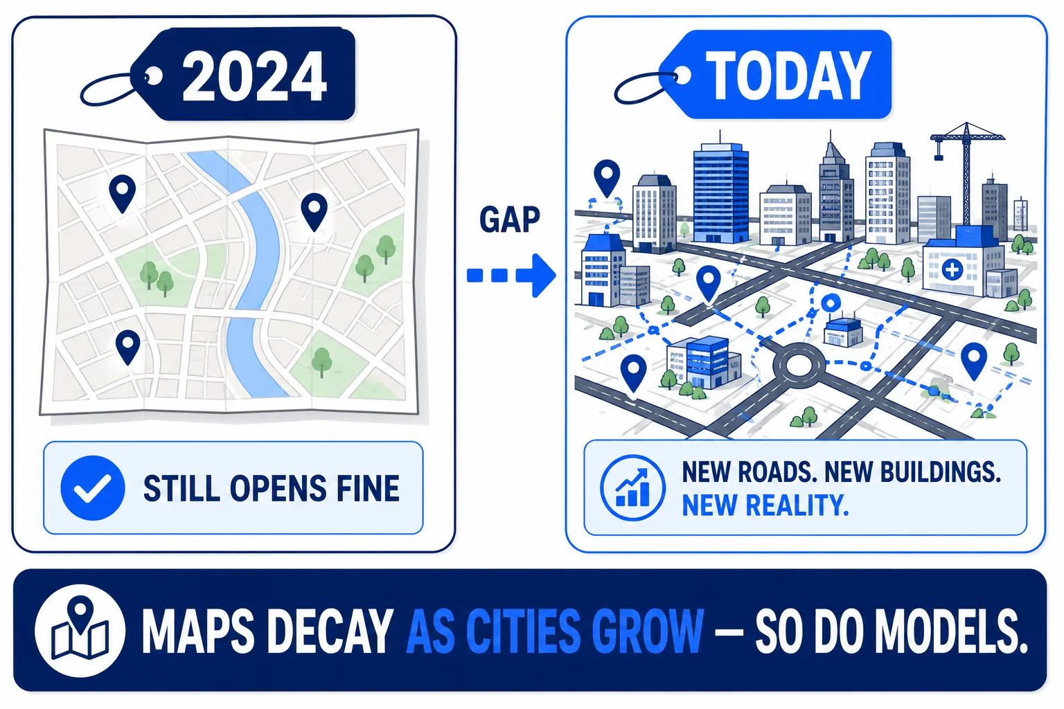
Start with one simple truth:
A model learns from the world of the past, but has to work in the world of today.
Picture the model as a city map.
The map was drawn in 2024 from the roads, buildings, and routes that existed then. Once drawn, the map stops there.
But the real city does not stop with it.
New roads, new shops, and new travel habits appear all the time.
The map is not “broken” — it still opens just fine. It just gradually matches the real world less and less.
Machine Learning models are the same.
When a model starts to decay — its quality dropping — there are usually two main causes: Data Drift and Concept Drift.
Data Drift — When the People Walking Through the Door Change#
Suppose a model predicts what products customers will buy.
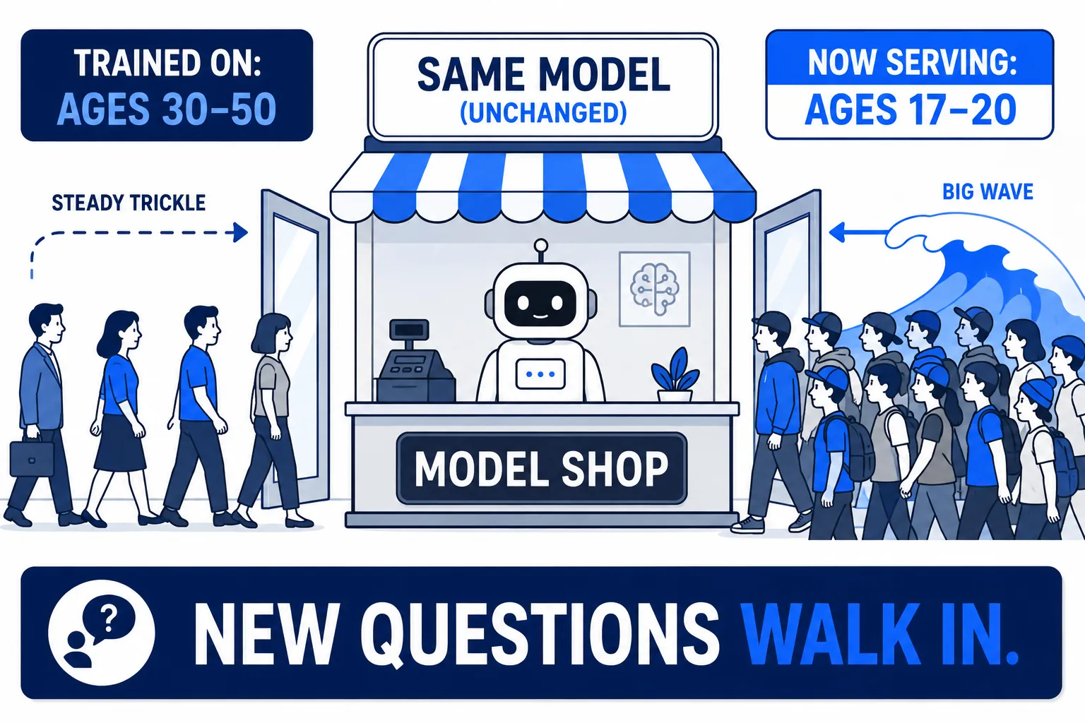
The training data came from 2024 customers, mostly aged 30–50.
The model learned that group’s behavior quite well.
One day marketing launches a hugely successful TikTok campaign.
Suddenly a large wave of 17–20 year-olds starts using the system.
The problem: the model barely saw this group during training.
It keeps answering predictions as usual — no errors, possibly even with high confidence.
But now it is being asked questions about a group of people it hardly knows.
This is Data Drift.
The inputs changed, but the model stayed the same.
Or simply:
Data Drift = new kinds of data walking through the door.
Concept Drift — Data Looks the Same, but the Meaning Changed#
Concept Drift is a little different.
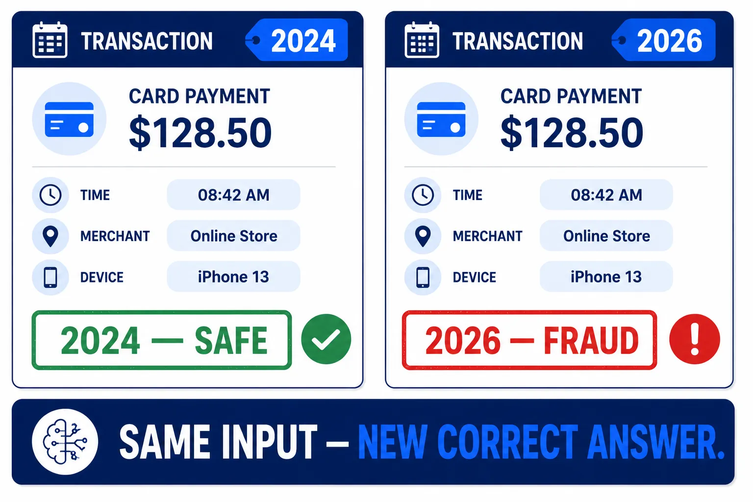
Suppose a fraud detection model was built in 2024.
It learned that transactions roughly like this are suspicious:
- several purchases in a row
- small amounts
- unusual hours
- a new device
Time passes, and fraudsters adapt.
Instead of many small transactions at odd hours, they switch to larger amounts, normal hours, and stolen accounts or devices.
Some of the data may still look like ordinary transactions the model has seen.
But the relationship between input and correct answer has changed.
A pattern that used to mean “safe” may now mean “fraud”.
This is Concept Drift.
Similar inputs, but the correct answer has changed.
To remember the difference in one line:
Data Drift = new questions. Concept Drift = new answers to the same questions.
1.9 The Scary Part: Both Happen Silently#
The server may still be running normally.
The API still answers:
200 OK
Latency still 30 ms. CPU still 40%. Error rate still 0%.
The infrastructure dashboards may be entirely green.
But the model’s predictions are quietly getting worse.
And the model itself cannot raise its hand to say:
“The data coming in lately doesn’t look like what I studied.”
Sometimes the truth only lands when the ground truth — the real answer — arrives days or weeks later.
For example, fraud detection says a transaction is safe today, and two weeks later the customer reports a stolen card. Only then is that prediction known to be wrong.
This is why the serving lifecycle must be a loop, not a straight line.
Train → Serve → Monitor → Retrain → Serve → Monitor → …
And it is why production ML needs more than a health check.
A health check asks:
“Is the server still up?”
Model monitoring asks:
“Is the model still doing well?”
These two questions are not the same at all.
A server can be 100% healthy while model quality drops every day.
So a real system needs request logging, prediction monitoring, and — once ground truth arrives — comparing it back against the predictions.
Because an API still being up does not mean the AI is still good.
2. Metrics That Match the Money#
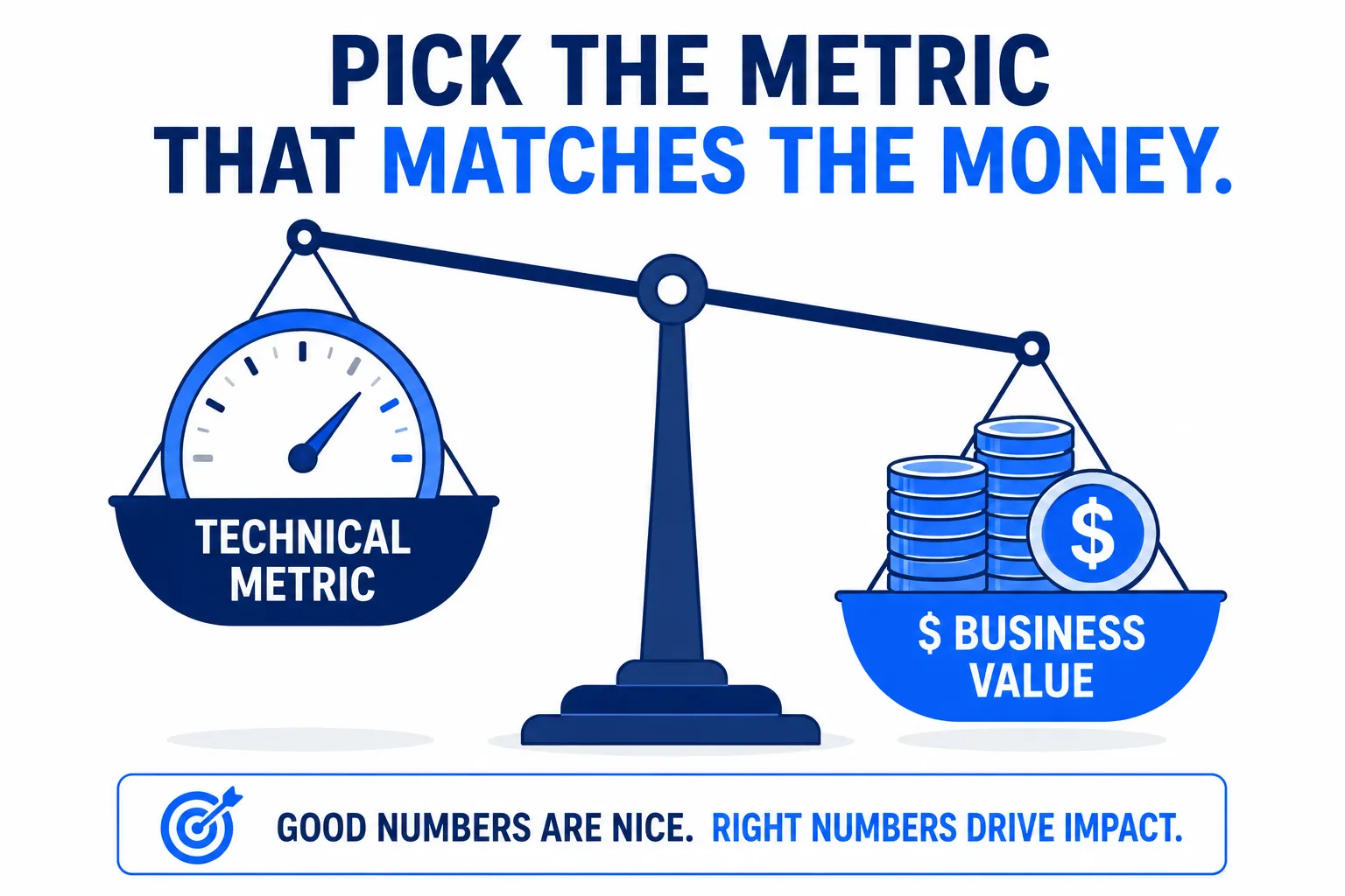
Another thing that changes when Machine Learning leaves the classroom: the best technical metric may not be the metric that matters most to the business.
2.1 Accuracy Lies When Data Is Imbalanced#
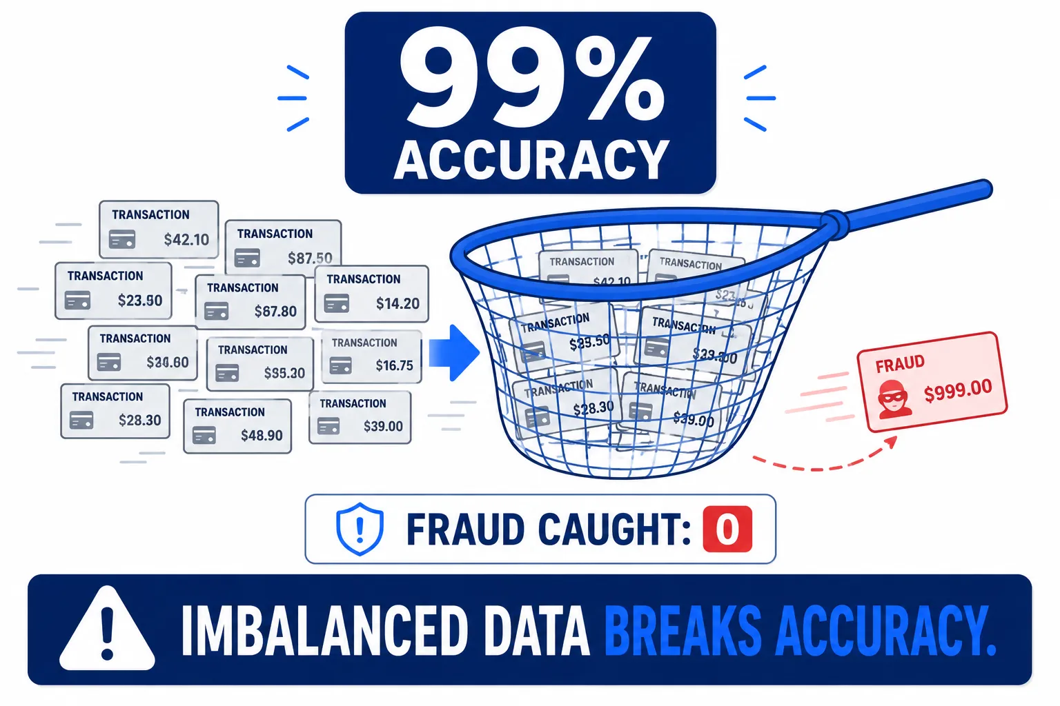
Start with the most familiar one: Accuracy.
Suppose there are 10,000 transactions, and only 1% — 100 of them — are fraud.
Build a simple “model” that answers the same thing every time:
“Not fraud.”
It is right 9,900 out of 10,000 times.
So:
Accuracy = 99%
Sounds wonderful.
But this model catches fraud:
0
Not a single one.
Prove it with fraud.csv:
amount,num_last_hour,new_device,night,fraud
120,2,0,0,0
45,1,0,1,0
8900,1,1,1,1
230,0,0,0,0
60,3,0,1,0
150,1,0,0,0
75,2,0,1,0
310,0,0,0,0
99,1,0,1,0import pandas as pd
from sklearn.dummy import DummyClassifier
df = pd.read_csv("fraud.csv")
X = df.drop(columns="fraud")
y = df["fraud"]
always_safe = DummyClassifier(strategy="most_frequent").fit(X, y)
print("accuracy :", always_safe.score(X, y)) # 0.888… (8 of 9)
print("fraud caught :", always_safe.predict(X).sum()) # 0Nine rows with only one fraud — answering “safe” every time scores high accuracy while catching zero fraud, a miniature of the 99% story above.
This is the problem with Accuracy when the data has class imbalance — when the number of examples per class differs wildly.
2.2 Confusion Matrix: See Every Way the Model Can Be Wrong#
Instead of looking at Accuracy alone, look at all four possible outcomes.
| Model says FRAUD | Model says SAFE | |
|---|---|---|
| Actually fraud | ✅ caught | ❌ missed fraud |
| Actually safe | ❌ false alarm | ✅ correct |
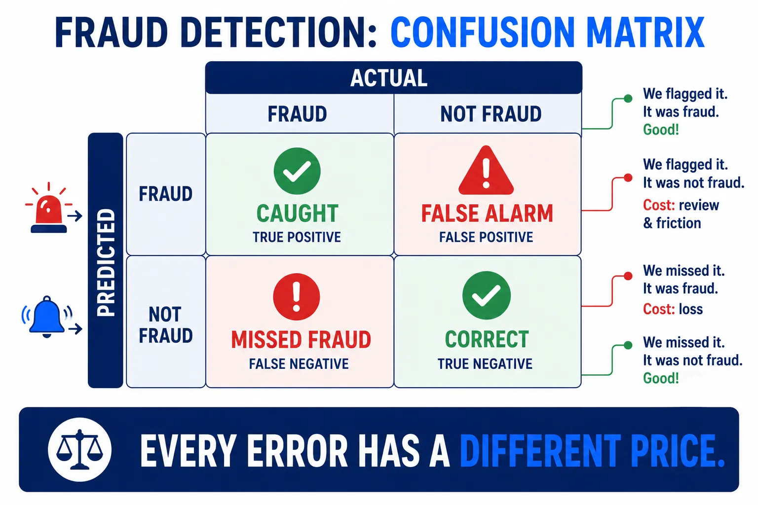
From here, two metrics matter: Precision and Recall.
Precision asks:
“Of every time the model raised a fraud alert, how many were actually fraud?”
High precision means alerts are usually right, with few false alarms.
Recall asks:
“Of all the fraud that actually occurred, what percentage did the model catch?”
High recall means little fraud slips through.
2.3 Picture a Fishing Net — Precision and Recall#
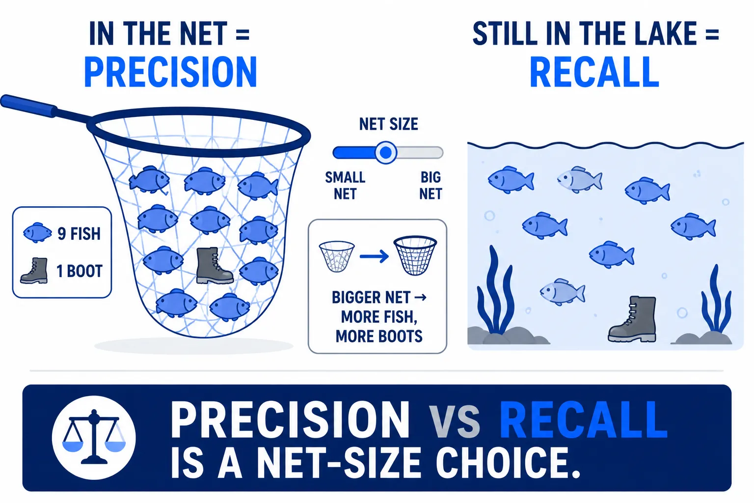
Imagine catching fish with a net in a lake.
Precision asks:
Of everything caught in the net, what percentage is actually fish?
If the net holds 9 fish and 1 boot, precision is excellent.
Recall asks:
Of all the fish in the lake, what percentage was caught?
To catch more fish, one way is a bigger net.
More fish get caught → Recall rises
But more other things get caught too → Precision may fall
This is the very common Precision–Recall trade-off.
2.4 Threshold Is the Dial That Tunes the Trade-off#
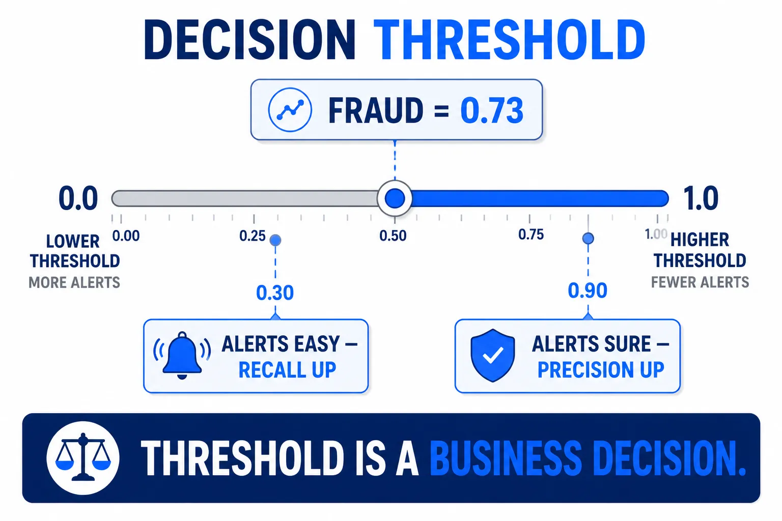
Most classification models do not start with the words Fraud or Safe.
They produce a score or probability, e.g.:
Fraud probability = 0.73
Then a Threshold is chosen:
if probability >= 0.50 → FRAUD
if probability < 0.50  → SAFE
Lower the threshold to 0.30,
and the model alerts more easily.
Recall usually rises, but false positives usually rise too.
Raise the threshold to 0.90,
and the model alerts only on very confident cases.
Precision usually rises, but some fraud slips through, so Recall falls.
So a threshold is not just a mathematical number — it is a business decision.
| Metric | Best when |
|---|---|
| Accuracy | Classes are fairly balanced and each kind of error costs about the same |
| Precision | False positives are expensive, e.g. blocking good customers |
| Recall | False negatives are expensive, e.g. missed fraud or missed disease |
| F1 Score | One number summarizing Precision and Recall is needed |
| ROC-AUC | Ranking/separation ability across many thresholds matters |
| RMSE / MAE | Regression — predicting a continuous number |
But more important than memorizing this table:
The business decides which kind of error is more expensive.
Say one missed fraud causes an average of $10,000 in damage.
But wrongly blocking one good customer might cost nothing more than a support call.
In that case, accepting more false positives in exchange for higher recall is the right call.
Because the real goal is not the prettiest metric.
It is lowering cost or creating value for the system as a whole.
2.5 A 30% Precision Model Can Still Make Money#
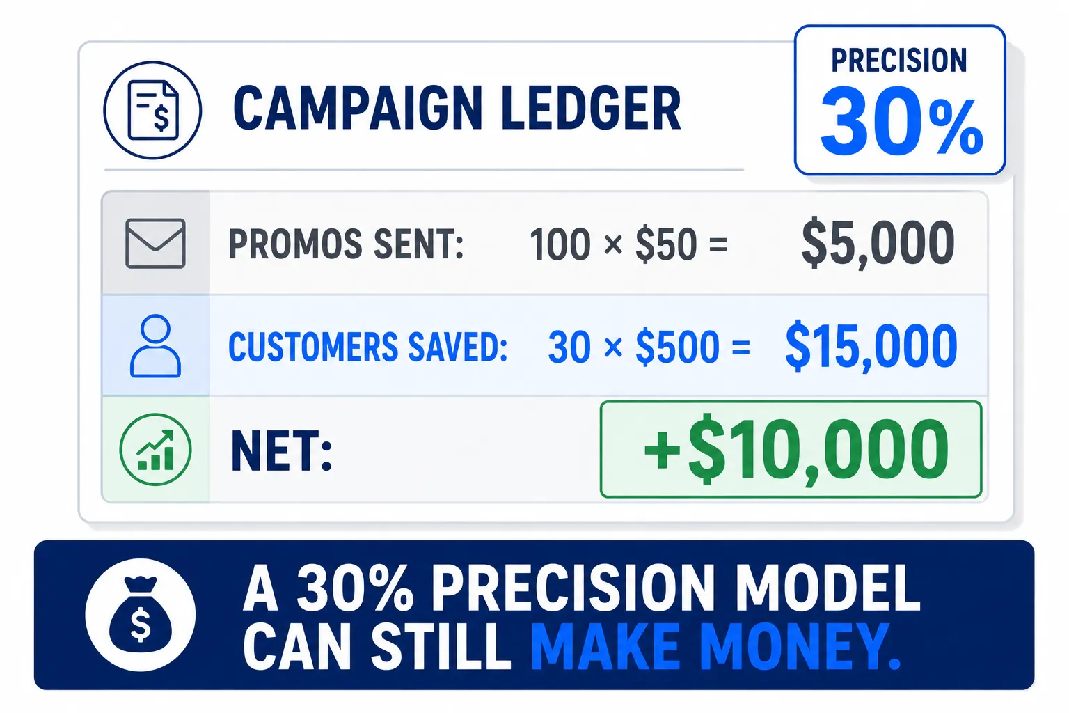
Suppose a customer churn model.
The model picks 100 customers likely to cancel, and the company sends each a $50 promotion.
The cost is:
100 × $50 = $5,000
It turns out that of those 100, only 30 were actually about to churn.
So Precision is just:
30 / 100 = 30%
Sounds bad.
But suppose each retained customer is worth $500.
The value retained is:
30 × $500 = $15,000
Minus the promotion cost:
$15,000 - $5,000 = +$10,000
A model with only 30% Precision just created $10,000 of net value.
This is why a model should never be chosen on a metric alone.
Metrics are not the final business goal — they are decision aids.
A model with beautiful metrics that creates no value may be useless.
Conversely, a model with ordinary-looking metrics that actually earns revenue, reduces damage, or saves cost may be the one worth deploying.
Summary#
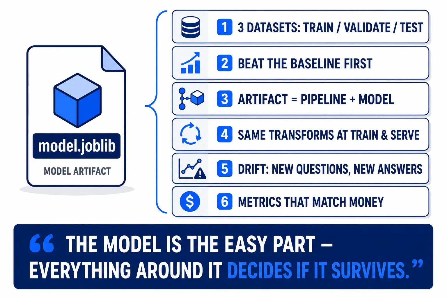
If only one sentence survives from this part, keep this one:
In production the exam never ends — the model keeps answering new questions forever, usually without an answer key, so the job shifts from scoring a model to watching one.
The map for this part, for reference:
- The exam never ends: every request is a fresh, unlabeled question — the ground truth arrives late or never, so production accuracy is far harder to see than a notebook score
- Fast and cheap count too: once
predict()lives inside an API, the trade-off becomes Prediction Quality ↔ Latency ↔ Cost — the most accurate model is not automatically the best one to ship - Overfitting vs. leakage: both look great in dev and fail for real — overfitting memorizes the training data (train good, test bad), leakage sees the answer key (train and test both suspiciously great)
- The one leakage question: for every feature ask “at the moment we must predict, is this value already known?” — if not, it must not be an input
- Models decay silently: Data Drift is new questions, Concept Drift is new answers to old questions — the server can stay green (
200 OK, low latency) while predictions quietly rot, so monitor the data, not just the box - Metrics tied to money: accuracy lies under class imbalance, Precision/Recall is choosing which error is more expensive, the threshold is a business dial — and a 30% precision model can still be worth deploying if the value it saves beats its cost