ML Refresher — Revisit ML Before Production
Set up Python, venv, Jupyter, then revisit ML before production — baselines, feature schemas, train/serve skew, drift, and business-aligned metrics
ML Refresher#
This article assumes you have already been through the basics of Machine Learning, so there will be no full ML course from scratch.
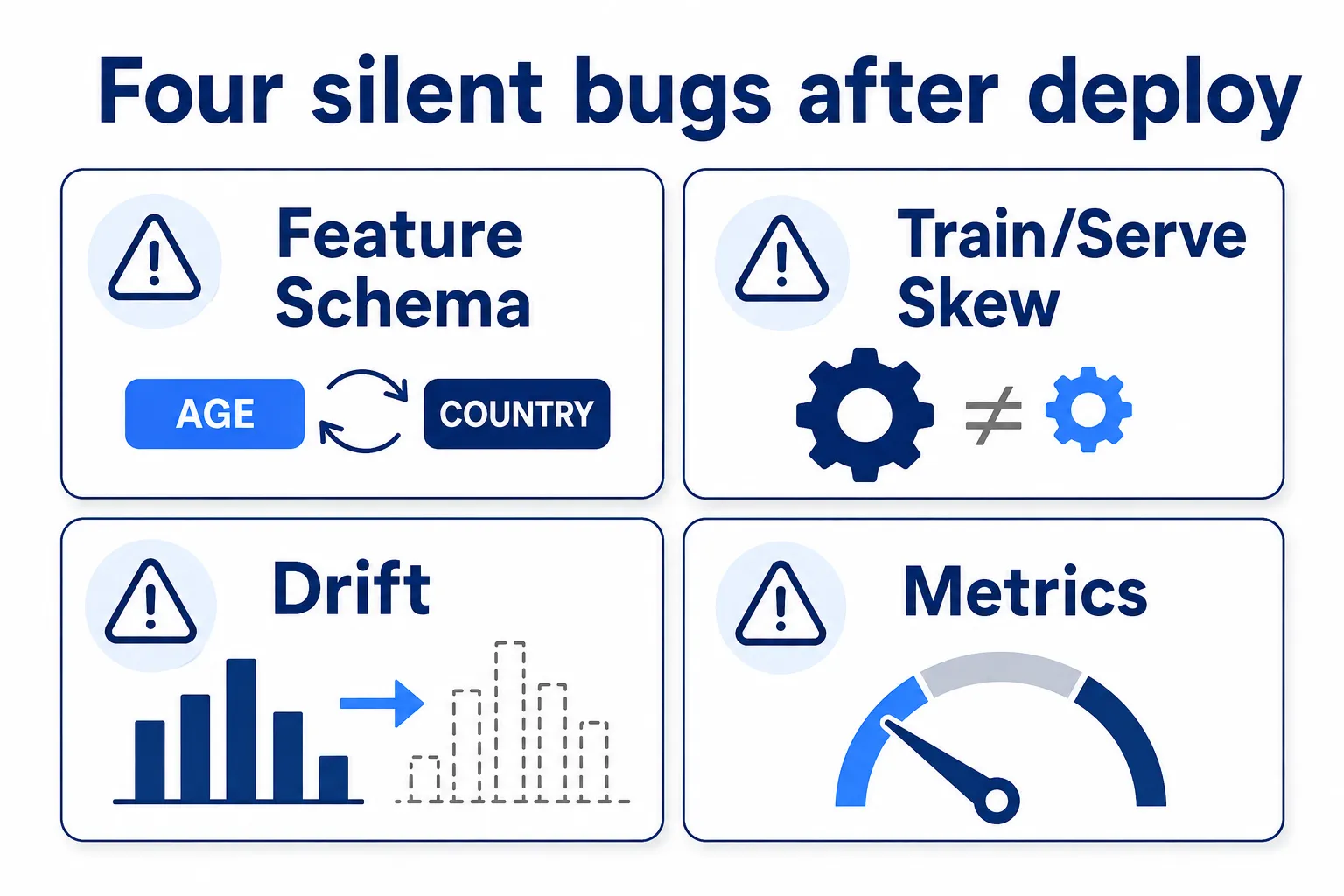
Only the concepts that matter when a model goes to production are reviewed, each viewed through one question:
What problem will this cause after deploy?
Because a model that works well in a notebook does not automatically keep working well once it serves real users.
And since every example in this article is designed to be followed along in a notebook, the first step is getting the tools ready.
1. Set Up the Tools First#
1.1 Install Python#
Download the installer at python.org/downloads ↗ and pick the latest Python 3.
On Windows, tick “Add python.exe to PATH” before clicking Install — otherwise python cannot be called from a terminal.
On Linux (Ubuntu), install it via apt:
sudo apt update && sudo apt install python3Then open a terminal and verify:
python --versionIf a version prints, e.g. Python 3.12.x, everything is fine (on Windows, if python doesn’t work, try py --version).
On Linux, use the
python3command, notpython— commands likepython3 --versionandpython3 -m venv .venv. The plainpythonmay not exist.
1.2 Create a Virtual Environment#
Why a Virtual Environment?
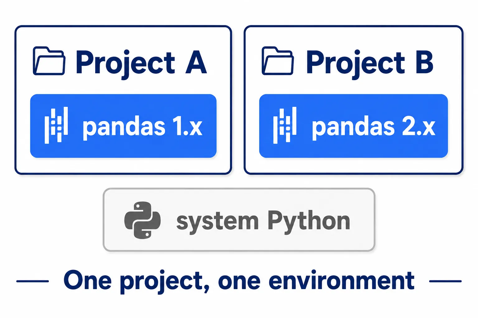
Installing every library into one shared machine-wide Python means that one day project A needs an old pandas while project B needs the new one — and everything starts breaking together.
A Virtual Environment creates a separate space for each project — installed libraries live inside that project’s own folder and never mix with other projects.
Create a project folder and run:
mkdir ml-refresher
cd ml-refresher

# create a virtual environment named .venv
python -m venv .venvThen activate:
Windows (PowerShell):
.venv\Scripts\activatemacOS / Linux:
source .venv/bin/activateOnce it works, (.venv) appears in front of the terminal prompt — the shell is now inside this project’s own space.
Activate again every time you come back to work. Use
deactivatewhen you want to leave the environment.
Note: if PowerShell warns about execution policy, run Set-ExecutionPolicy -ExecutionPolicy RemoteSigned -Scope CurrentUser once, then activate again.
1.3 Install Jupyter Notebook, pandas, and Friends#
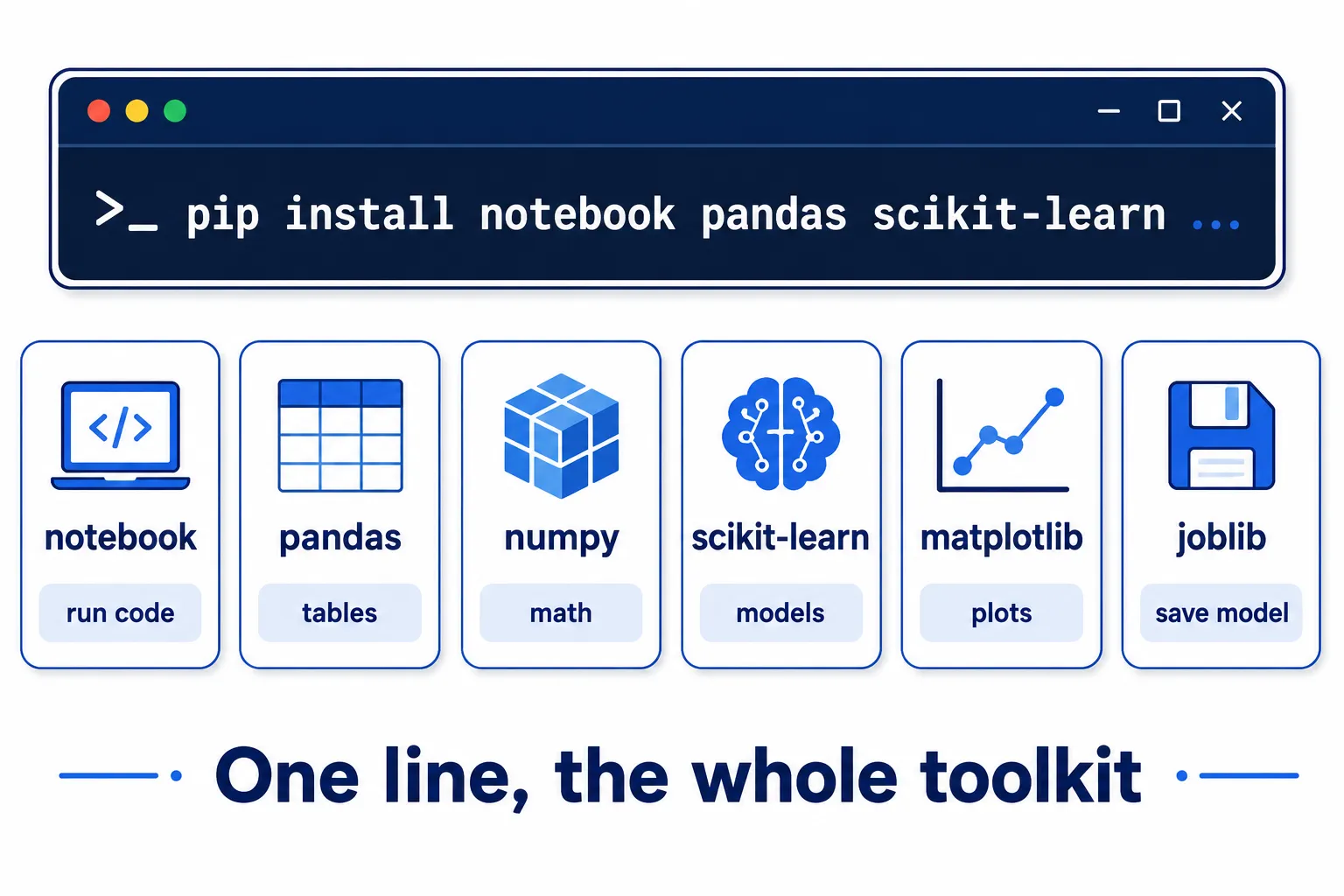
While (.venv) is visible, install every library used in this series:
pip install --upgrade pip

pip install notebook pandas numpy scikit-learn matplotlib joblibWhat each one does:
| Library | What it is for |
|---|---|
| notebook | Installs Jupyter Notebook — write and run code chunk by chunk, ideal for ML experiments |
| pandas | Tabular data handling (DataFrame) — read CSV, clean data, reshape |
| numpy | Array math — the foundation under pandas and scikit-learn |
| scikit-learn | The main ML library — preprocessing, models, and evaluation |
| matplotlib | Plot data distributions and results |
| joblib | Save a trained model as an artifact file (.joblib) |
1.4 Open Jupyter Notebook#
jupyter notebookThe browser opens Jupyter by itself. Create a new notebook (New → Python 3) and run a first cell to confirm everything installed:
import sys
import pandas, numpy, sklearn, matplotlib, joblib

print(sys.version)
print("pandas       ", pandas.__version__)
print("numpy        ", numpy.__version__)
print("scikit-learn ", sklearn.__version__)If the versions print without errors, the machine is ready.
1.5 Pin the Environment with requirements.txt#
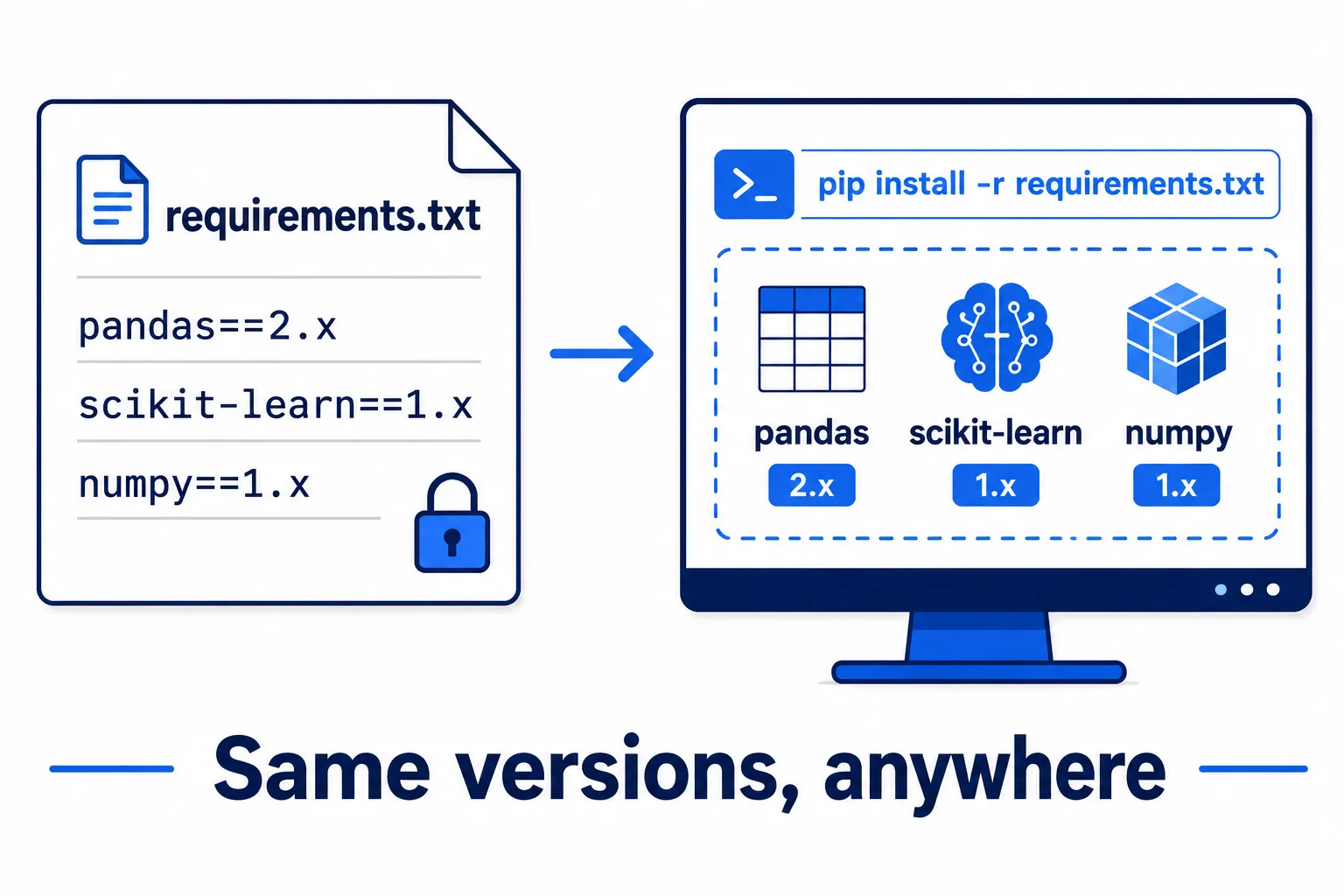
Another habit worth starting on day one:
pip freeze > requirements.txtThis file records the name and version of every library in the current environment. Anyone — including your future self, or a production machine — can rebuild the exact same environment with:
pip install -r requirements.txtNotice this is the same idea as Model Artifact versioning from before — it is not only the model that needs a known version. The environment that trained the model must be recorded and tracked the same way.
Tools are ready. Now on to the Machine Learning concepts that matter in production.
2. Machine Learning Basics, Revisited#
2.1 Supervised Learning Is Still the Main Tool#
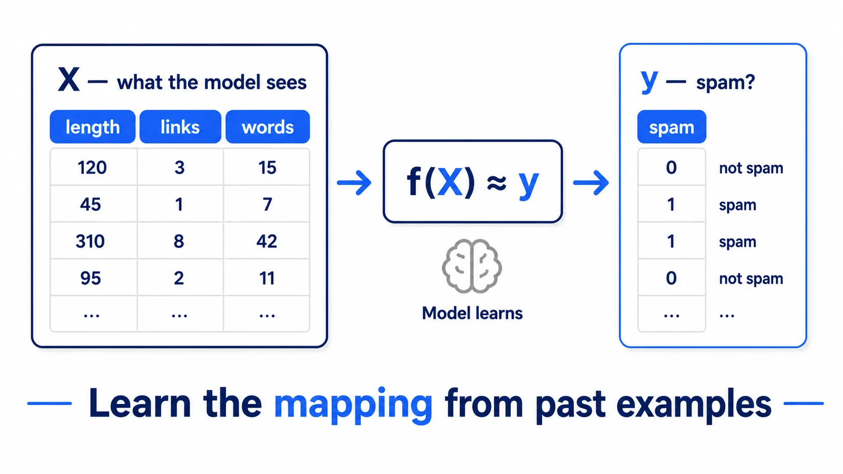
Supervised Learning means learning from past examples whose answers are already known.
Two ingredients matter:
-
X — Features the input data shown to the model, e.g. email length, number of links, sender domain, or counts of certain words
-
y — Labels the correct answer for each example, e.g.
spamornot spam
Put simply:
X = the data the model looks at y = the answer the model should learn
To make this tangible, one small example file runs through the whole article — create spam.csv in the same folder as the notebook (just copy and save it):
length,num_links,num_capital_words,sender_domain_new,spam
420,0,1,0,0
380,1,0,0,0
510,0,2,0,0
290,0,0,0,0
600,1,2,0,0
440,0,1,0,0
350,1,0,0,0
470,0,2,0,0
530,3,8,1,1
400,0,0,0,0Read it with pandas:
import pandas as pd

df = pd.read_csv("spam.csv")
print(df.shape)   # (10, 5)
dfIn this file, X is the first 4 columns and y is the spam column (0 = not spam, 1 = spam).
The job of a Machine Learning algorithm is to learn the relationship between these two.
Shorthand:
f(X) ≈ y
Or in plain words:
“Given data like X, what should y be answered?”
If y is a group or category, the task is called Classification.
For example:
Email → Spam / Not Spam
But if y is a continuous number, it is called Regression.
For example:
house data → house price
2.2 What About Other Kinds of Machine Learning?#
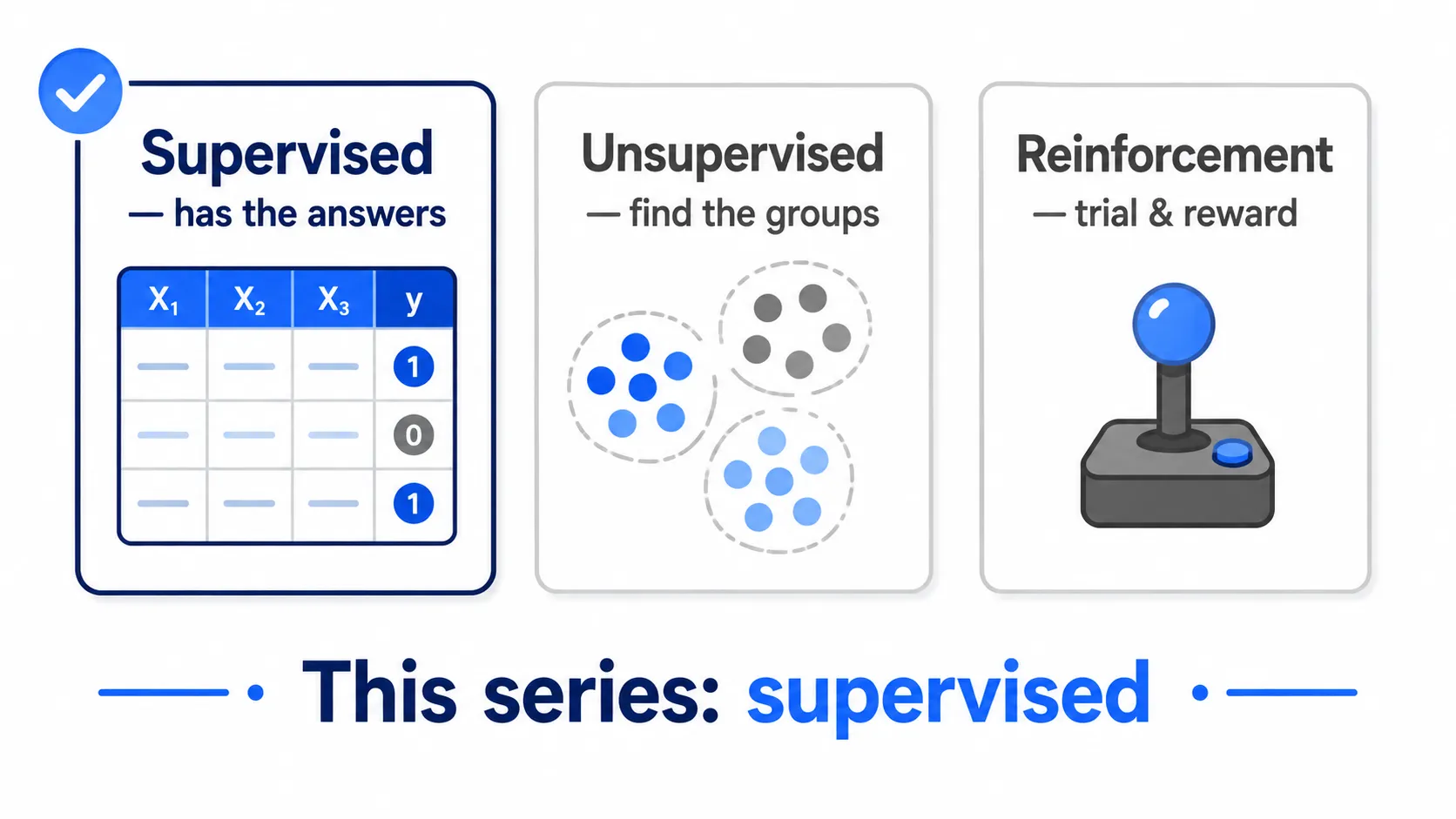
Broadly speaking, Machine Learning comes in three kinds:
- Supervised Learning — examples with answers (both X and y exist); learn from the past to predict the future
- Unsupervised Learning — only X, no answers; find patterns or groups, e.g. customer segmentation or anomaly detection
- Reinforcement Learning — learn by trial and error with rewards and penalties, e.g. robotics or game-playing AI
This series focuses on Supervised Learning.
Because most organizational ML that has to run in production as a service is a task with known answers — is it fraud, will the customer cancel, what should the price be.
And the problems ahead — schema, skew, drift, monitoring — happen to every kind just the same.
2.3 Train / Validation / Test — Why Three Sets#
A first Machine Learning course usually splits data only two ways: Training and Test.
Real work needs three sets:
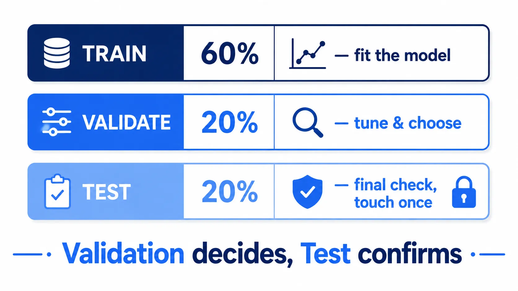
- Training Set — used to fit the model
- Validation Set — used to score while developing, tune hyperparameters, and choose which model is best
- Test Set — measured once, at the end, to confirm the final result
Why a separate Validation set?
Because every time results from a set are used to make decisions — say, try 20 models and keep the one with the best score — that set stops being data the model has “never seen”.
The resulting score partly reflects the selection across many tries, not the model’s true ability.
import pandas as pd
from sklearn.model_selection import train_test_split

df = pd.read_csv("spam.csv")
X = df[["length", "num_links", "num_capital_words", "sender_domain_new"]]
y = df["spam"]

# first split: lock the Test set away
X_train_val, X_test, y_train_val, y_test = train_test_split(
    X, y, test_size=0.2, random_state=42
)

# second split: carve Validation out of what remains
X_train, X_val, y_train, y_val = train_test_split(
    X_train_val, y_train_val, test_size=0.25, random_state=42
)So the rule is one line:
Validation may decide many times. Test is used once — and that once is the last.
With little data, Cross-Validation is an alternative: split the data into k parts and rotate which part serves as validation. It gives steadier numbers when data is limited.
This theme returns in production — the real data flowing at the model every day is a test set that never ends and arrives without an answer key.
2.4 Always Start With a Baseline#
Before training anything complex, there is one step beginners tend to skip and practitioners almost never do: building a Baseline.
A baseline is the simplest possible way to answer the task — so simple it looks dumb.
For a spam detection task where 90% of email is not spam, the simplest baseline is “always answer not spam.”
In scikit-learn it takes a few lines:
import pandas as pd
from sklearn.dummy import DummyClassifier

df = pd.read_csv("spam.csv")            # 9 of 10 rows are not spam
X = df.drop(columns="spam")
y = df["spam"]

baseline = DummyClassifier(strategy="most_frequent")  # answers the most frequent class every time
baseline.fit(X, y)
print(baseline.score(X, y)) # 0.9 — always saying "not spam" already scores 90%For a regression task like house prices, a baseline may simply be “always answer the average price of all houses.”
Two benefits:
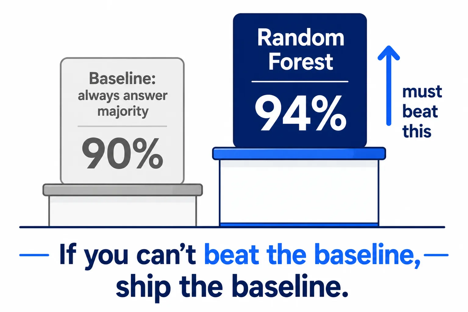
First — it is the line every model must beat.
If Random Forest gets 94% while a dumb baseline gets 90%, the complex model adds only 4 points of real value. If it cannot do even that, there is no reason to ship that complexity to production.
Second — it guards against self-deception.
An accuracy number means nothing without something to compare against. 94% sounds impressive, but if the baseline is 92%, the model barely gained anything from the data.
If you can’t beat the baseline, ship the baseline — cheaper, faster, and easier to maintain.
2.5 Classical ML Is Still Everywhere#
These days, “AI” evokes Deep Learning, Neural Networks, or LLMs first.
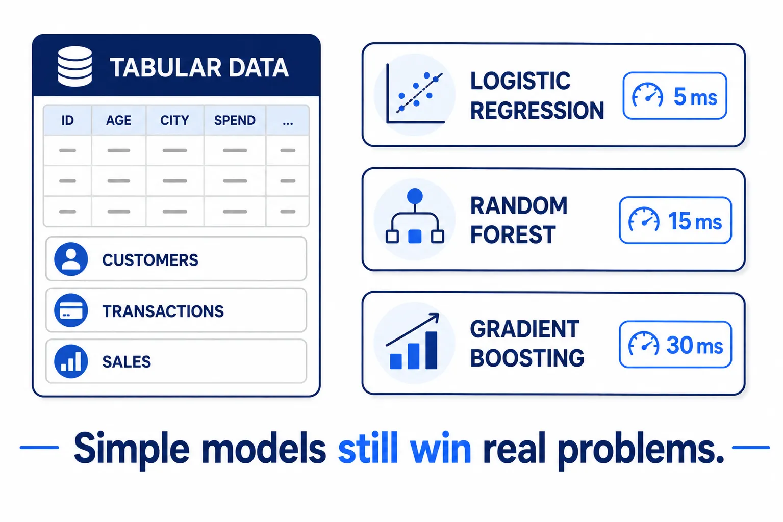
But in real systems, Classical Machine Learning such as
- Logistic Regression
- Random Forest
- Gradient Boosting
is still widely used — especially on tabular data, the rows-and-columns kind: customer records, transactions, sales, products, and business-system data.
For many tasks, a large Neural Network is simply unnecessary.
Simpler models come with real advantages: fast to train, light on resources, easy to deploy, and quick to answer.
And for this series, that simplicity is a feature.
Random Forest will therefore be the main model for learning serving.
Not because Random Forest is the best model for every problem, but because the real subject is everything around the model.
The path to watch:
Train → Save → Deploy → API → Predict → Monitor → Retrain
If Random Forest answers a prediction in a few milliseconds, every serving lesson here works exactly as it would with a large Neural Network that takes longer and needs more hardware.
The goal is not to build the most complex model — it is to learn how to put a model to real use.
Importantly, these ideas are not tied to Random Forest.
Logistic Regression, XGBoost, Neural Networks, computer-vision models, or even an application calling an LLM through an API — much of the thinking stays the same:
There is input → a model → a prediction → a serving system → and whatever happens after deploy must be monitored.
Models may change; the problems of running Machine Learning in the real world remain.
3. Three Terms to Know Before Production#
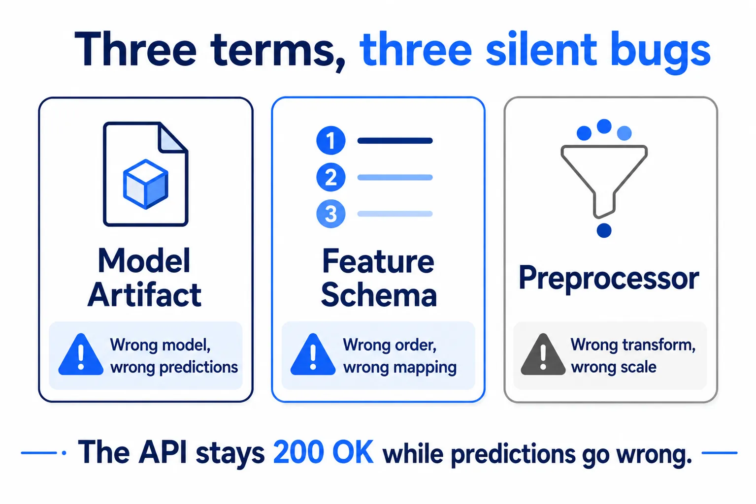
Before going further, three terms must be rock solid, because many production ML problems do not arrive as a crashed server or a red error.
They arrive as the system still running, the API still answering 200 OK, and the predictions being wrong.
And that is more dangerous than a visible error.
The three terms: Model Artifact, Feature Schema, and Preprocessor.
3.1 Model Artifact — the Model Saved as a File#
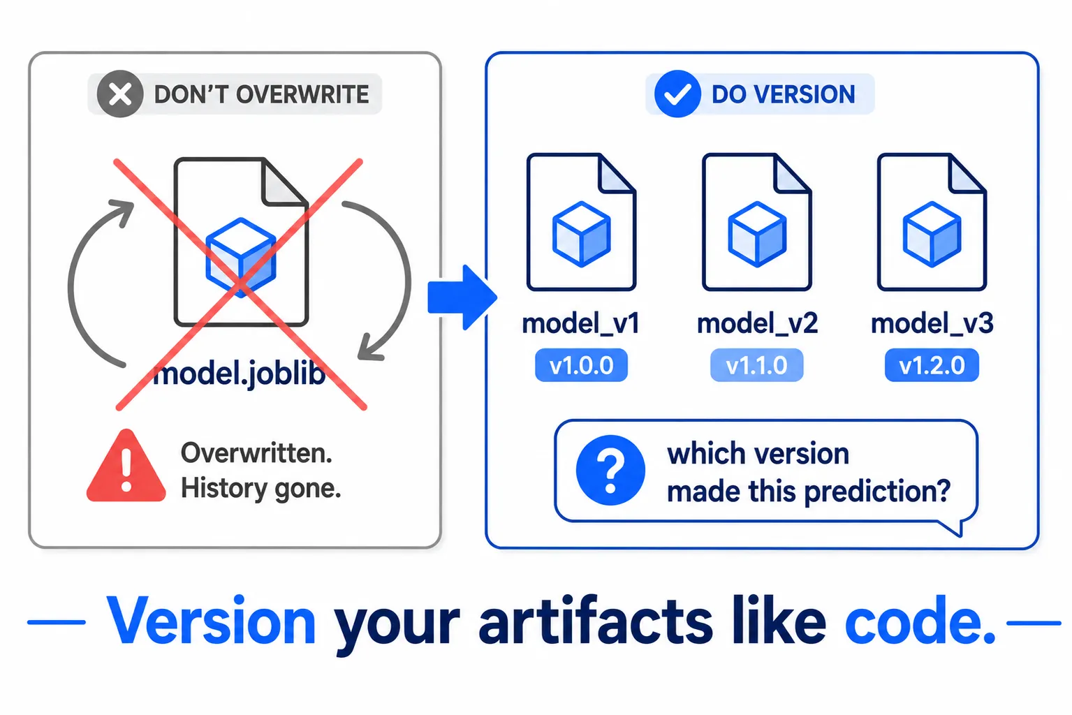
This term already appeared in the previous part.
After training, the model is serialized and saved to a file such as:
model.joblib
That file is the Model Artifact — what the server loads for prediction.
Artifacts deserve management as serious as source code, especially versioning.
Instead of a single file named:
model.joblib
overwritten again and again, production should always know which version it is running, e.g.:
model_v1.joblib
model_v2.joblib
model_v3.joblib
Because one day someone will ask:
“Which model version made this prediction?”
Without an answer, debugging or auditing past results becomes very hard.
3.2 Feature Schema — the Model Must Know What Each Input Slot Is#
Suppose a model is trained with features in this order:
[age, income, days_since_signup]
The model therefore learns:
- the first value is
age - the second value is
income - the third value is
days_since_signup
Try it with a real file — create customers.csv in the same folder as the notebook:
age,income,days_since_signup,will_buy
25,30000,10,0
52,78000,200,1
34,45000,55,0
45,62000,120,1
23,28000,5,0
61,90000,300,1
29,36000,30,0
58,84000,260,1Then train a model with exactly this column order:
import pandas as pd
import joblib
from sklearn.ensemble import RandomForestClassifier

df = pd.read_csv("customers.csv")
X = df[["age", "income", "days_since_signup"]]   # this order matters a lot
y = df["will_buy"]

model = RandomForestClassifier(random_state=0).fit(X, y)
joblib.dump(model, "model_v1.joblib")But at serving time, the program sends:
[income, age, days_since_signup]
The number of features is unchanged. The data types are still numbers, same as before. No value is missing.
So the program may not error at all.
The problem is the model now reads income as age and age as income.
And keeps predicting confidently.
# Serving side sends a swapped order — no error, no exception, wrong answer
wrong_order = [[62000, 45, 120]]   # actually [income, age, days_since_signup]
model.predict(wrong_order) # answers 0 — but this customer's true answer is 1No error, no exception — just wrong predictions.
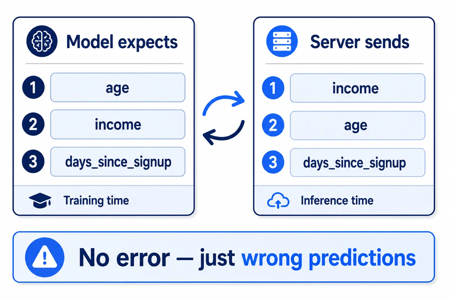
This is why a Feature Schema matters.
It must be explicit what the model expects:
Which features → in what order → with what data types
And the serving side must send data matching what the model saw during training.
3.3 Preprocessor — What Happens to the Data Before It Reaches the Model#
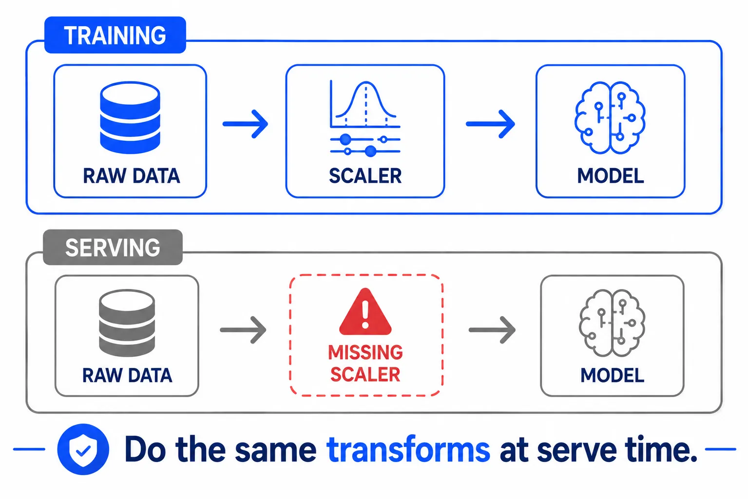
Raw data rarely goes straight into a model.
Some preprocessing usually happens first, such as:
- scaling numbers
- filling missing values
- encoding categories
- converting text to numbers
Suppose training used a StandardScaler to transform the data before the model.
The training flow is:
Raw Data → Scaler → Model
But once deployed to production, the serving program does this instead:
Raw Data → Model
The scaler step was forgotten.
The model now receives data shaped differently from what it saw during training.
And the problem is it may not error.
It can still compute and return a prediction — just a possibly very wrong one.
When the data preparation during training and serving differ, it is called Train/Serve Skew.
The principle is simple:
Whatever you do to the data during Training, do exactly the same during Serving.
3.4 The Better Way: Save a Pipeline, Not Just a Model#
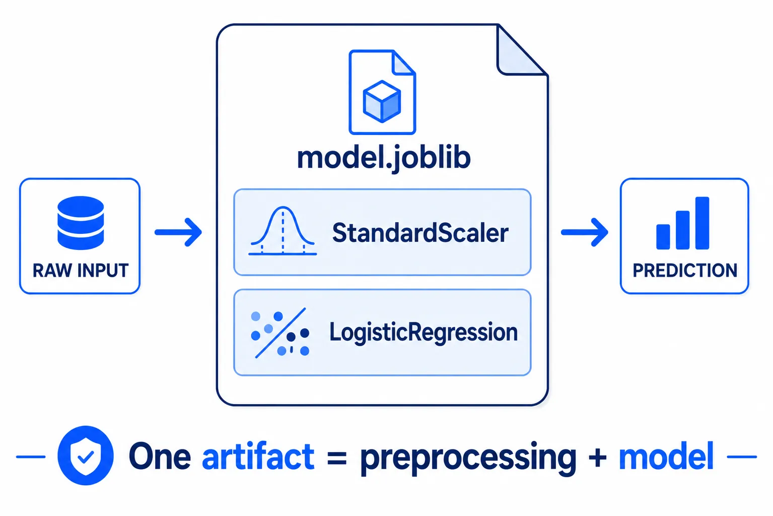
Instead of hoping the serving program remembers to call the scaler first every time, the preprocessor and model can be bundled together.
In scikit-learn, that is done with a Pipeline.
import pandas as pd
import joblib
from sklearn.model_selection import train_test_split
from sklearn.pipeline import Pipeline
from sklearn.preprocessing import StandardScaler
from sklearn.linear_model import LogisticRegression

df = pd.read_csv("customers.csv")                      # same file as the earlier example
X = df[["age", "income", "days_since_signup"]]
y = df["will_buy"]
X_train, X_test, y_train, y_test = train_test_split(X, y, test_size=0.25, random_state=42)

pipe = Pipeline([
    ("scale", StandardScaler()),      # step 1: scale the data
    ("clf", LogisticRegression()),    # step 2: feed it to the model
])

pipe.fit(X_train, y_train)

joblib.dump(pipe, "model.joblib")The key point: model.joblib no longer stores only the Logistic Regression.
It stores:
Scaler + Model
together in a single artifact.
So at serving time, all it takes is:
pipe = joblib.load("model.joblib")

prediction = pipe.predict([[52, 78000, 200]]) # order [age, income, days_since_signup]When predict() is called, the pipeline handles everything:
Input → StandardScaler → Logistic Regression → Prediction
The serving side no longer needs to remember “scale before predicting.”
That step is baked into the artifact back at training time.
This is a foundational design principle of ML serving:
Never leave correctness to human memory if the system design can enforce it.
Rather than writing one training pipeline and then trying to replicate it on the serving side, build one pipeline and serialize everything together.
The artifact becomes the single source of truth for how data is transformed and how predictions are made.
And that kills several forms of train/serve skew at the root.
The three silent bugs to remember:
| Watch out for | What goes wrong when missed |
|---|---|
| Model Artifact | No one knows which model version made a prediction |
| Feature Schema | Features arrive reordered or malformed, and the system still runs |
| Preprocessor | Training and serving transform data differently → train/serve skew |
All three cases share one thing:
The system may not break — the answers do.
And that is why production ML has to care about more than whether the API opens or the server is still up.
Summary#
If only one sentence survives from this part, keep this one:
Getting a model to run is the easy half — getting it to keep giving correct answers is the real work, and that work starts before you ever deploy.
The map for this refresher, for reference:
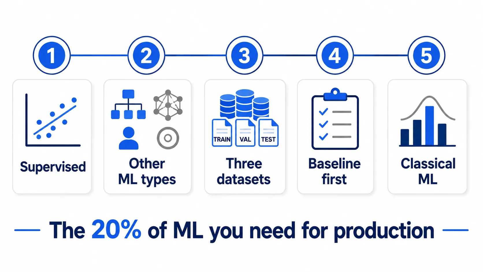
- Set up once, reproducibly: a per-project
venvplus a pinnedrequirements.txt, so the exact environment can be rebuilt anywhere — the training environment is an artifact too, not just the model - Three datasets: train fits, validation decides (and may be consulted many times), test confirms once at the very end
- Baseline first: measure the dumbest possible method, because a complex model only earns production if it clearly beats that line
- Classical ML still wins on tables: Random Forest and friends are fast, cheap, and enough for most tabular problems — the hard part is everything around the model, not the model
- Three silent bugs: Model Artifact (which version answered?), Feature Schema (right features, right order, right types), Preprocessor (the transforms applied before the model)
- One pipeline, one artifact: bundle preprocessing and model into a single
Pipelineso serving can never forget a step — this kills train/serve skew at the root
That is where the next part picks up — what changes once a model goes to production: the never-ending exam, overfitting vs. leakage, drift and decay, and the metrics that actually match the money.